Exploring data I
Lecture 4
2026-01-26
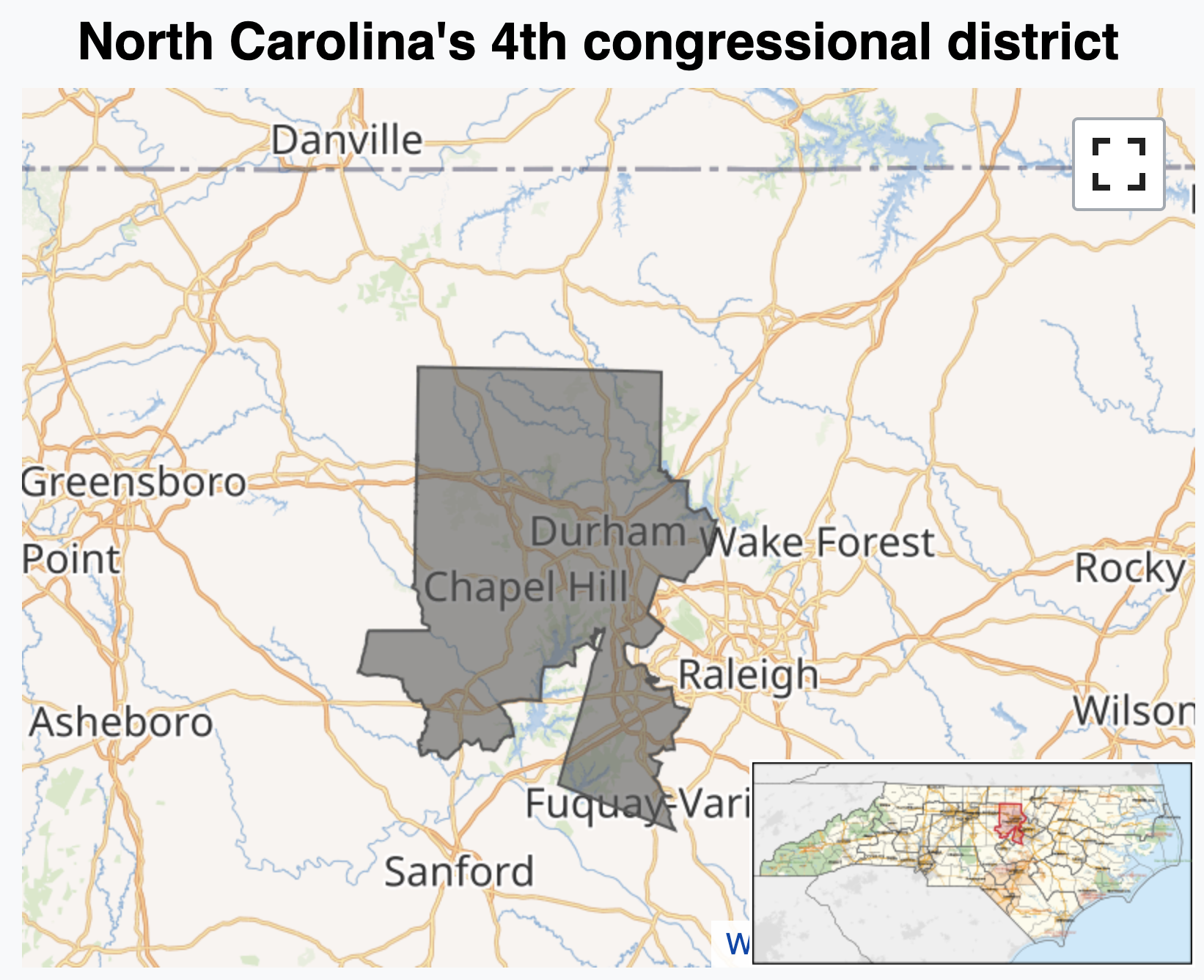
JZ’s tour of the USA
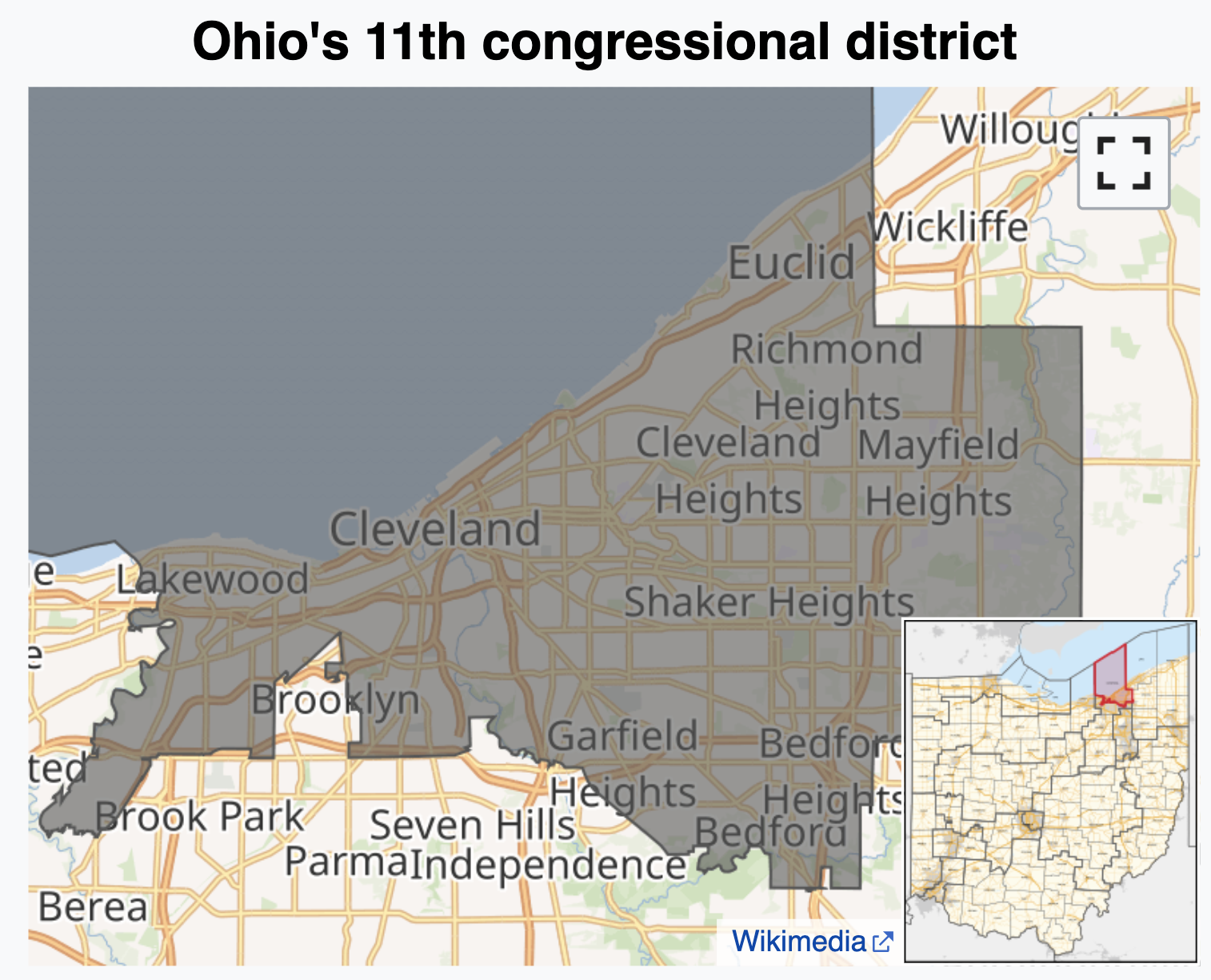
JZ’s tour of the USA
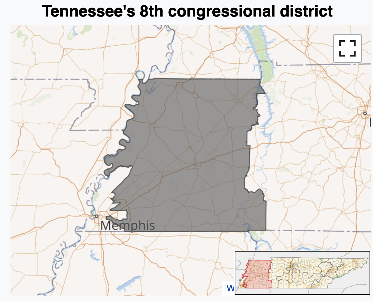
JZ’s tour of the USA
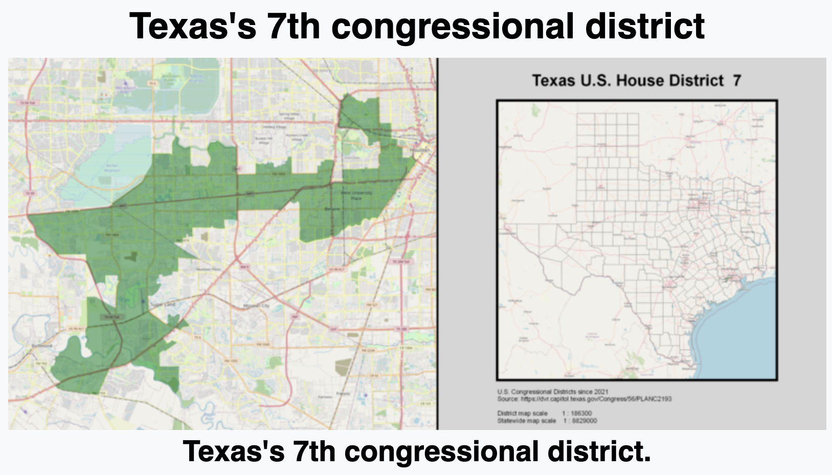
JZ’s tour of the USA
Histogram - Step 1

Histogram - Step 2

Histogram - Step 3
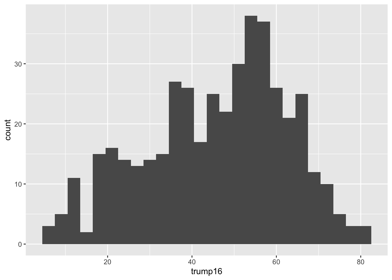
`stat_bin()` using `bins = 30`. Pick better value `binwidth`.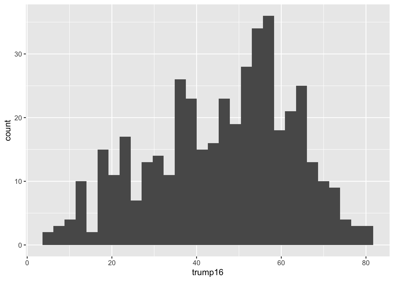
Histogram - Step 4
Histogram - Step 4
Histogram - Step 4
Histogram - Step 4
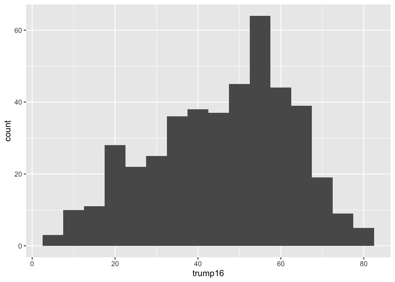
Histogram - Step 5
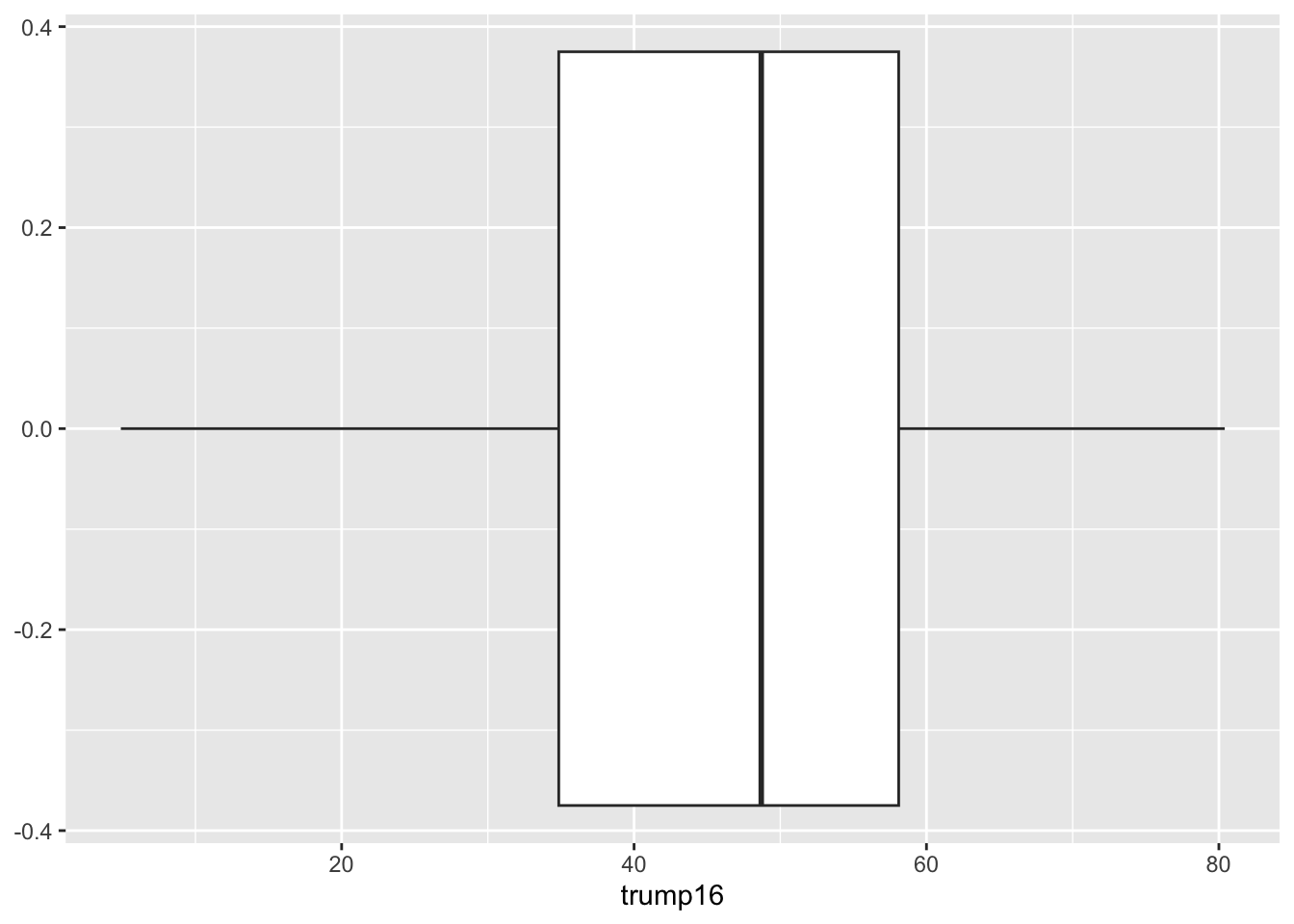
Box plot - Step 1

Box plot - Step 2
Box plot - Step 3
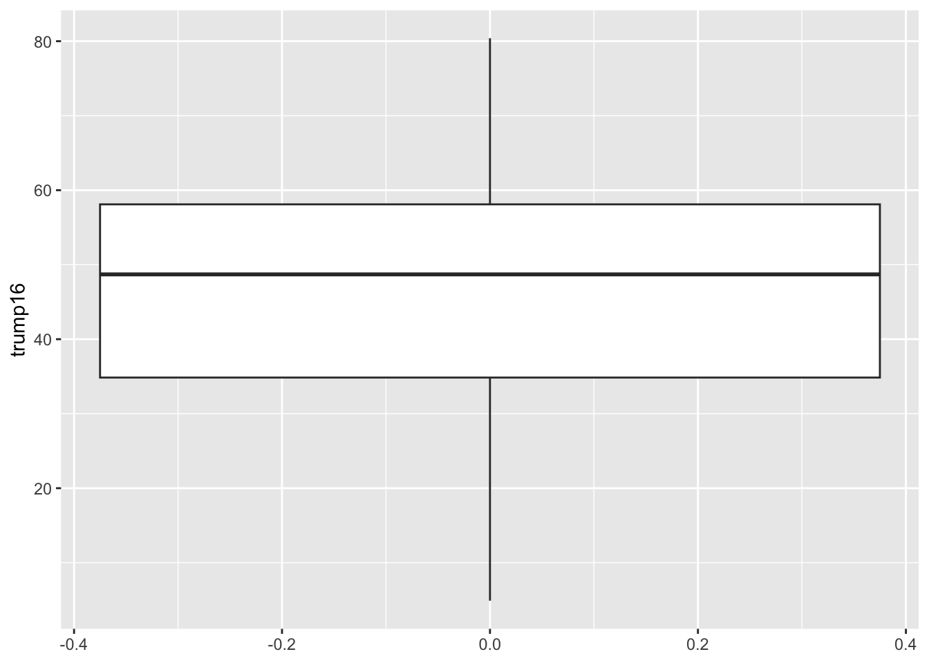
Box plot - Alternative Step 2 + 3
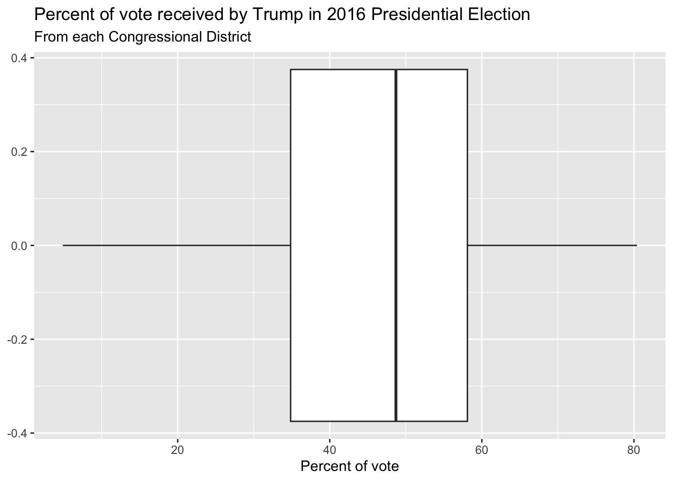
Box plot - Step 4
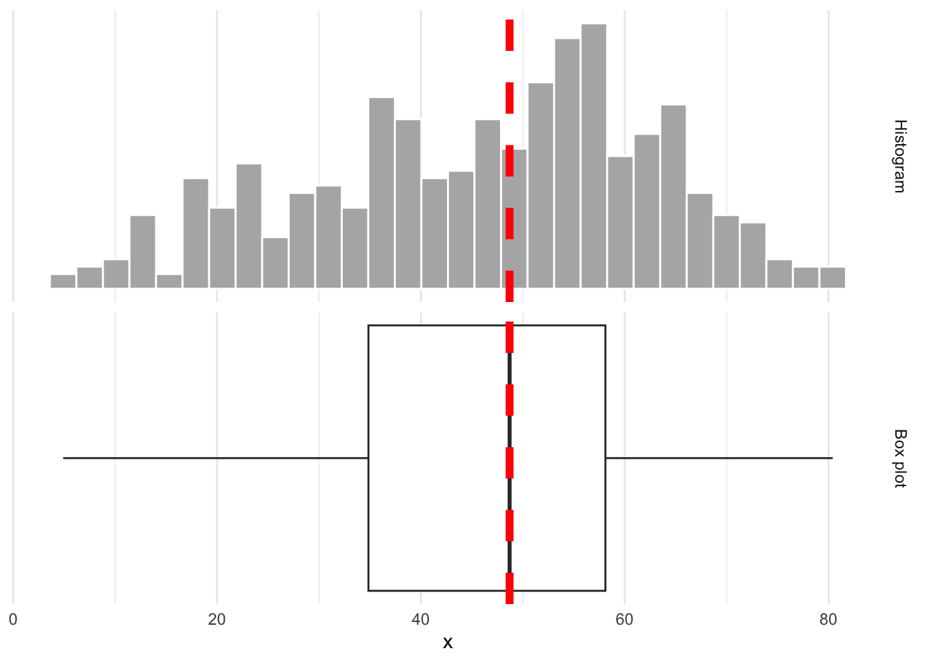
Whence the box?
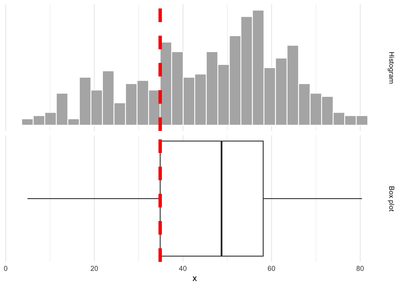
The middle of the box is the median. 50% of the data are below, and 50% are above:
Whence the box?
The lower edge of the box is the 25% quantile. 25% of the data are below, and 75% are above:
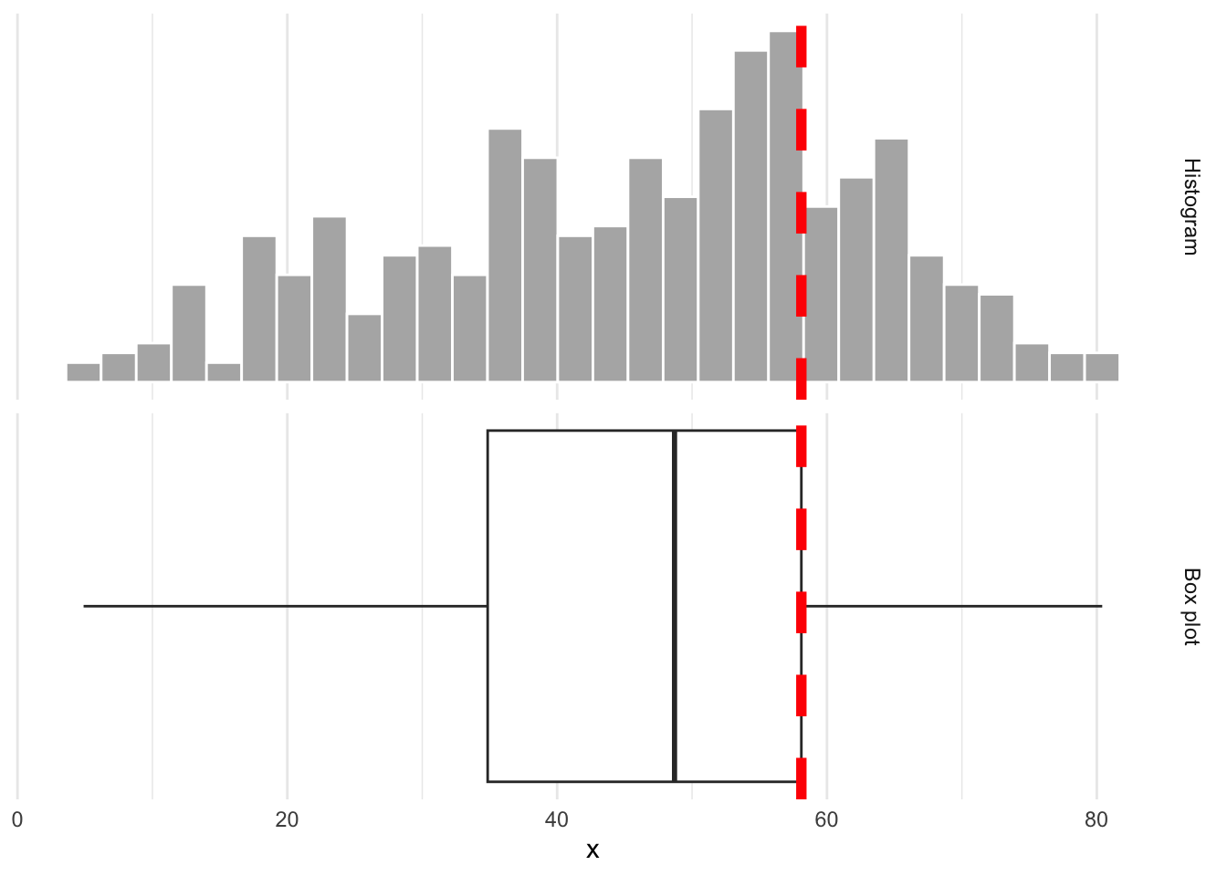
Whence the box?
The upper edge of the box is the 75% quantile. 75% of the data are below, and 25% are above:
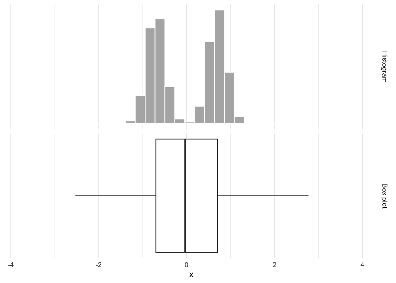
Box plots obscure modality
Same box plot:
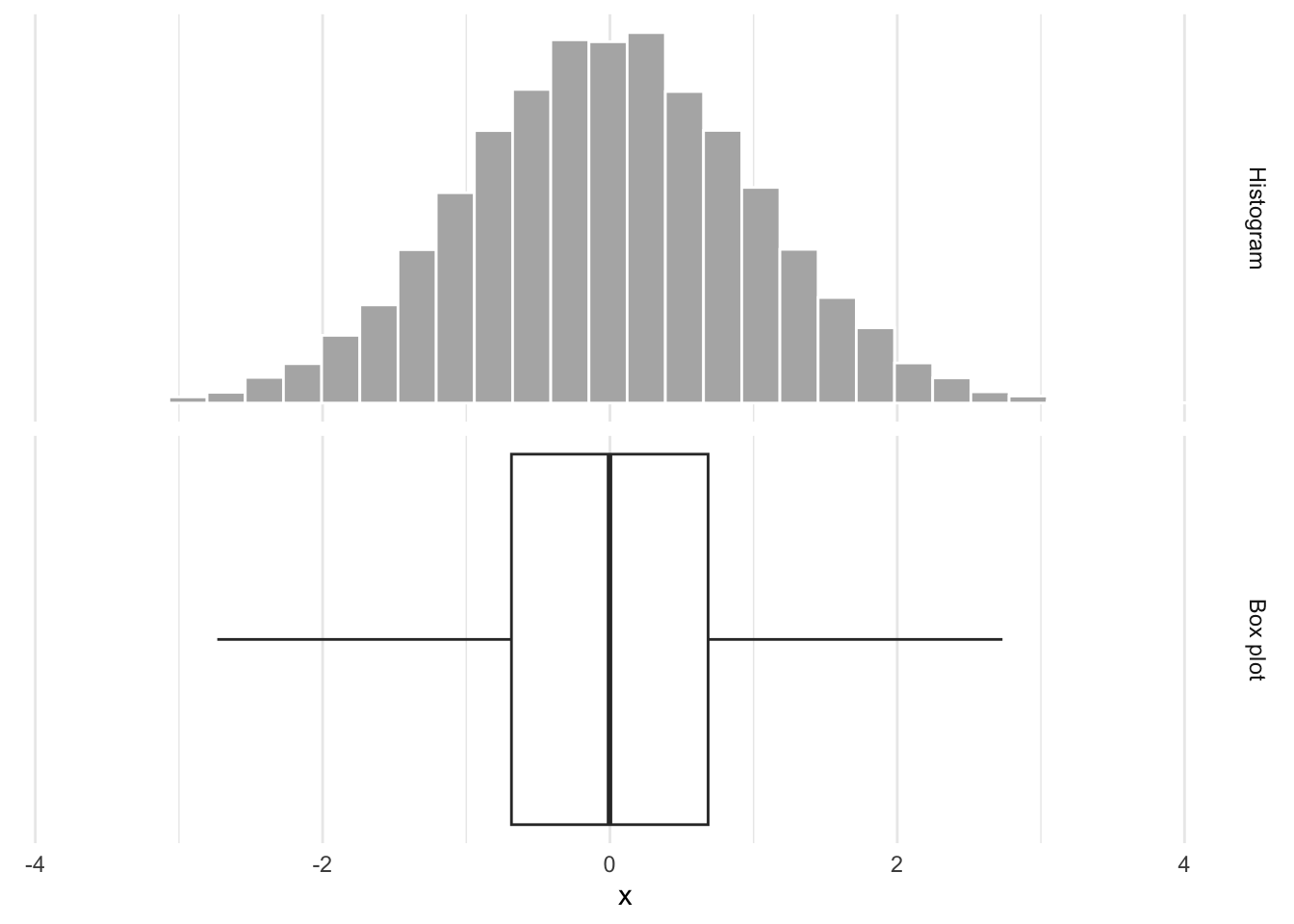
Box plots obscure modality
Very different distributions:
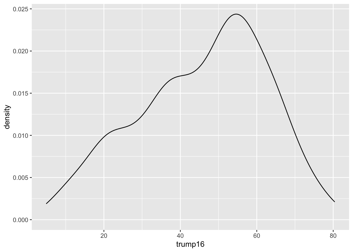
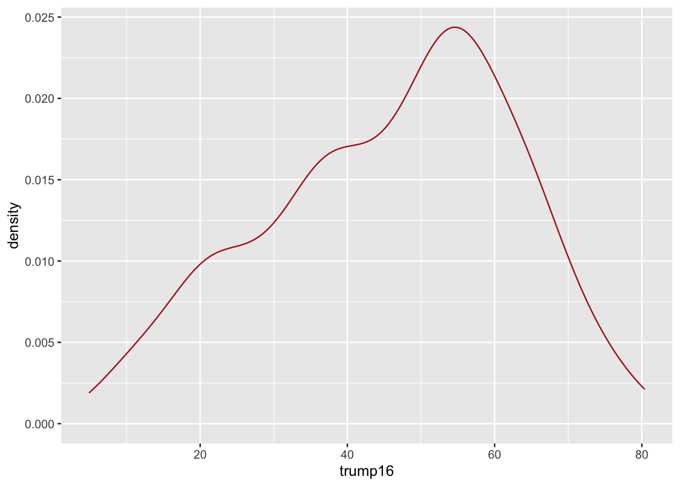
Density plot - Step 1

Density plot - Step 2

Density plot - Step 3
Contrast that with the histogram
ggplot(gerrymander, aes(x = trump16)) +
  geom_histogram(aes(y = after_stat(density))) +
  geom_density(color = "red")
`stat_bin()` using `bins = 30`. Pick better value `binwidth`.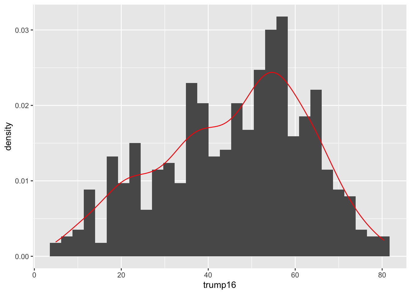
Prettier. Smooths out the lumps and bumps. There are still defaults you could learn to override.
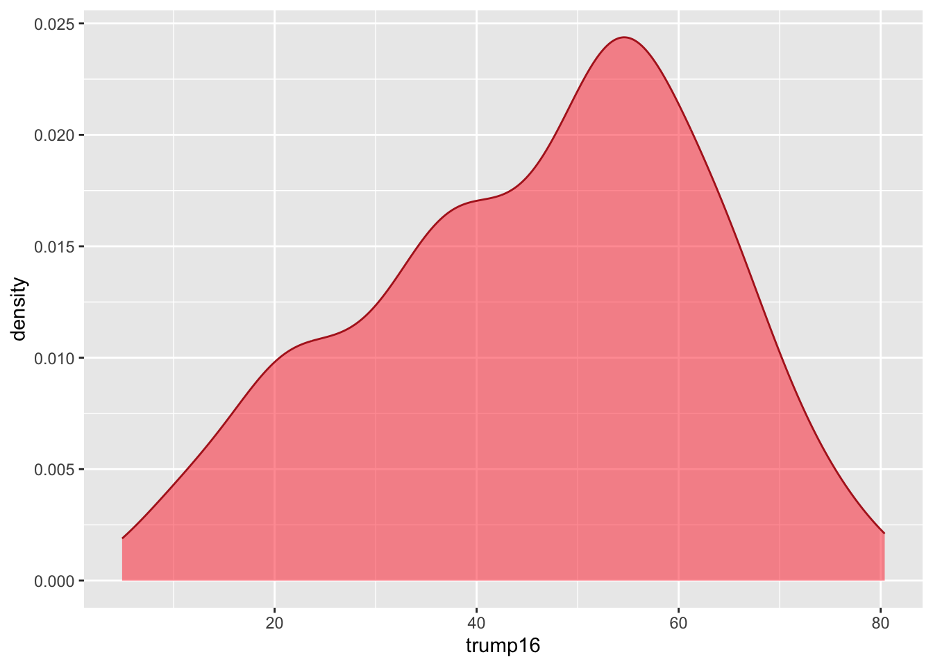
Density plot - Step 4
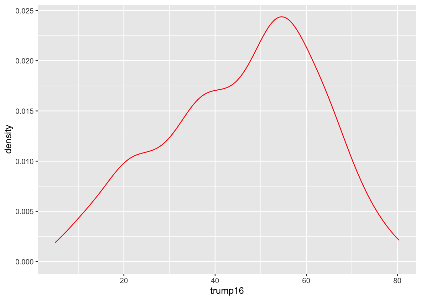
Density plot - Step 5
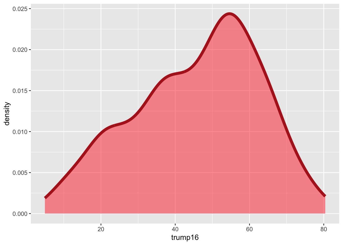
Density plot - Step 6

Density plot - Step 6
Density plot - Step 6
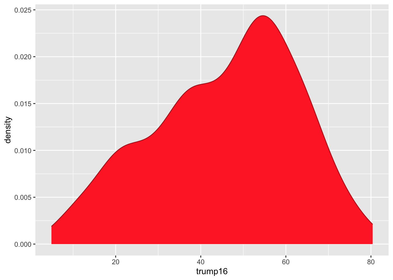
Density plot - Step 7
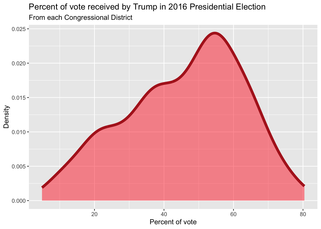
Density plot - Step 8
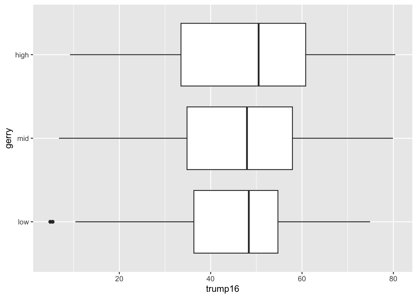
Side-by-side box plots
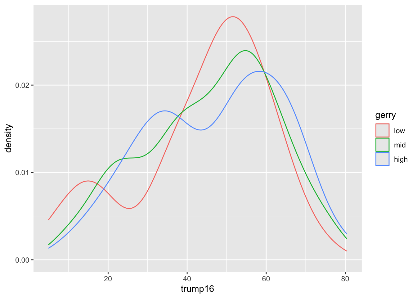
Density plots
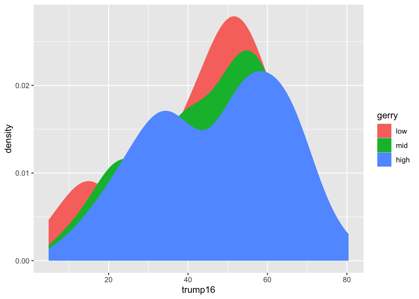
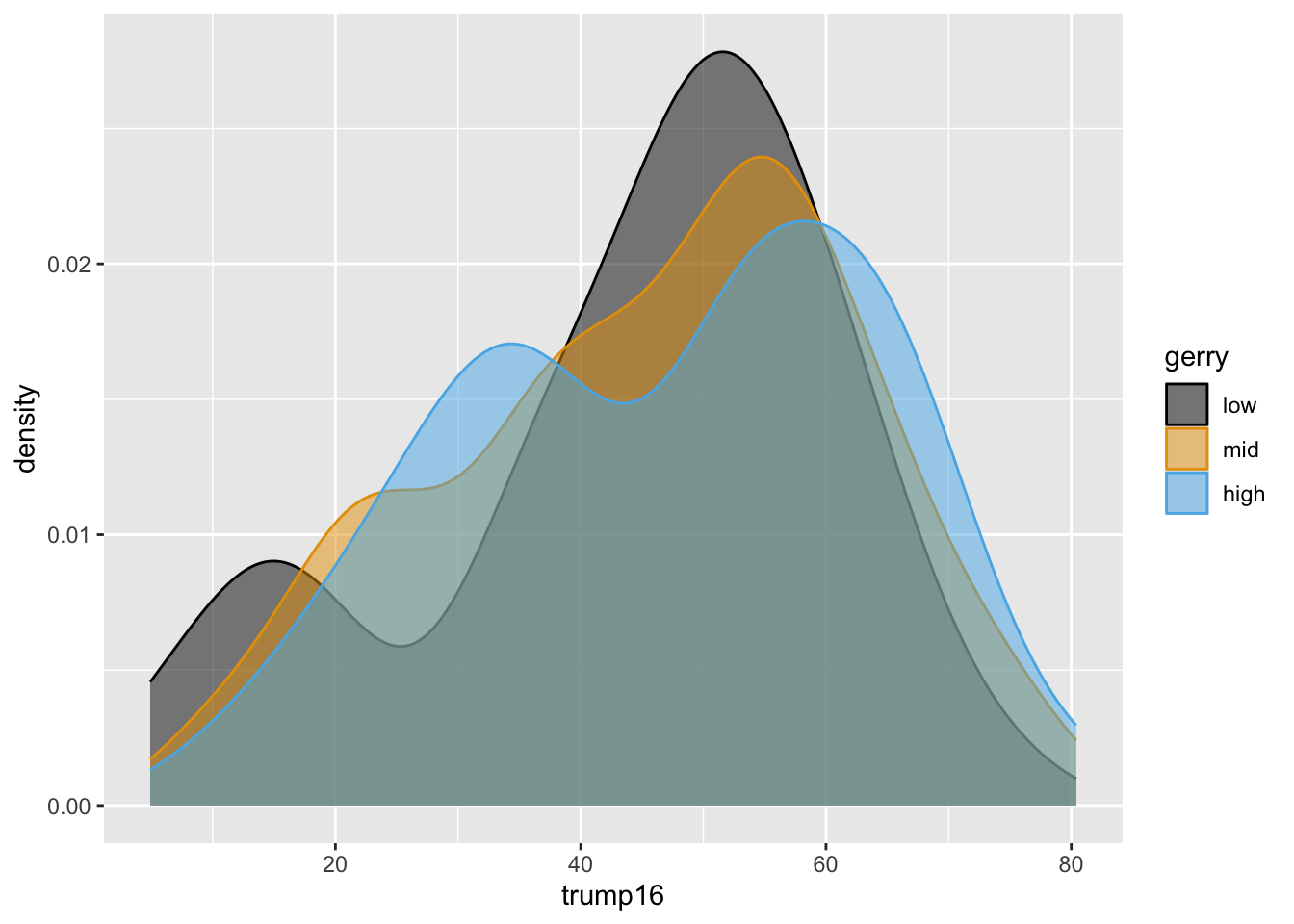
Filled density plots
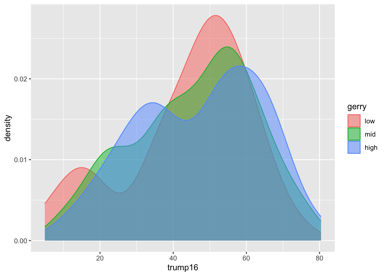
Better filled density plots
Better colors
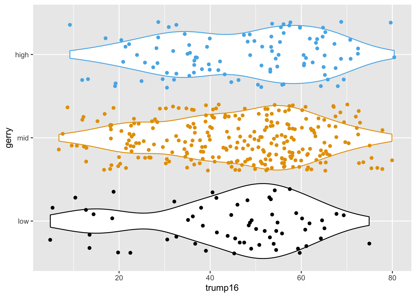
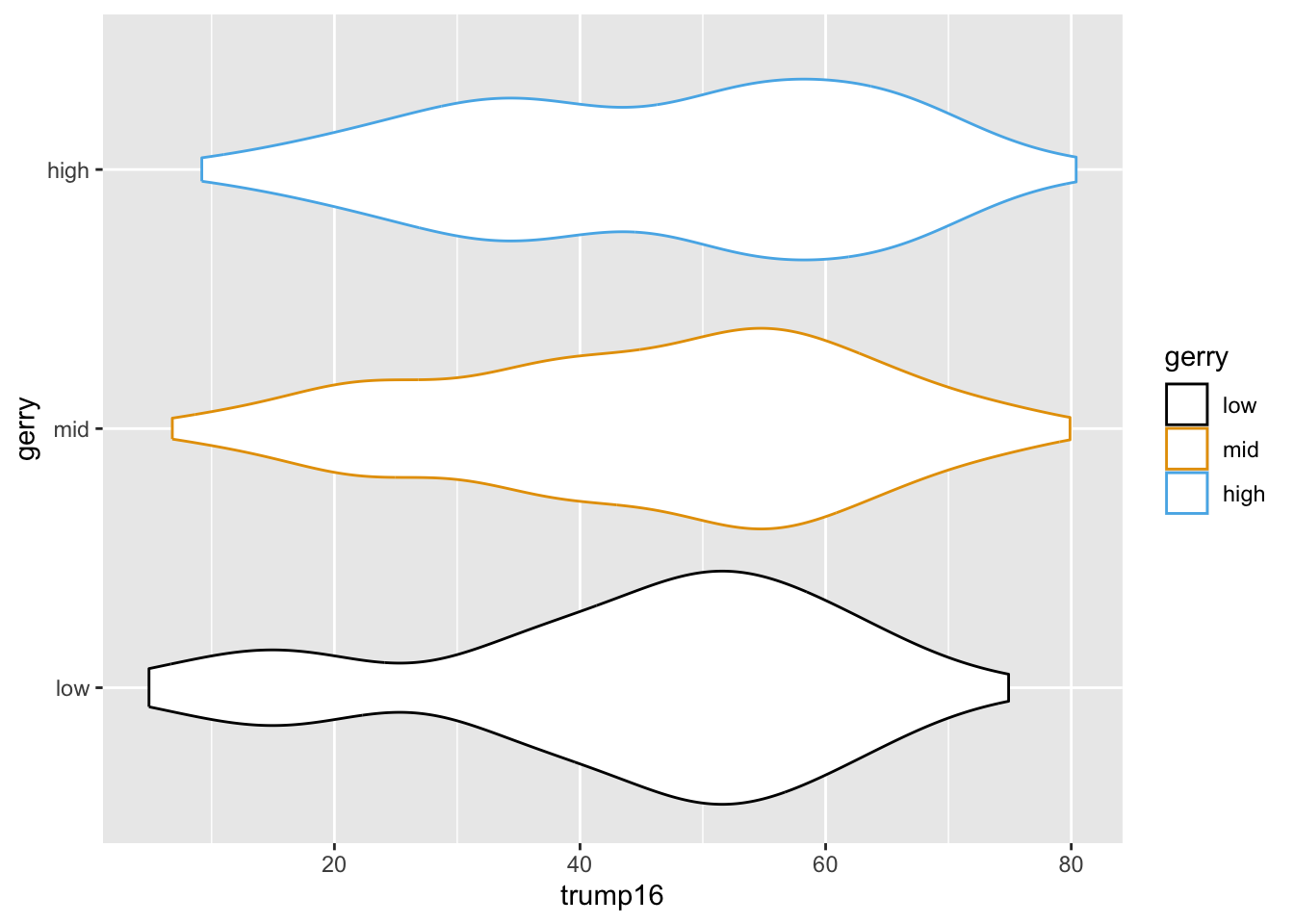
Violin plots
Multiple geoms
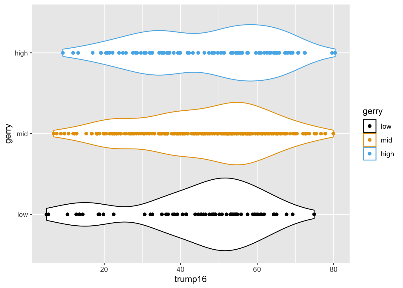
Multiple geoms
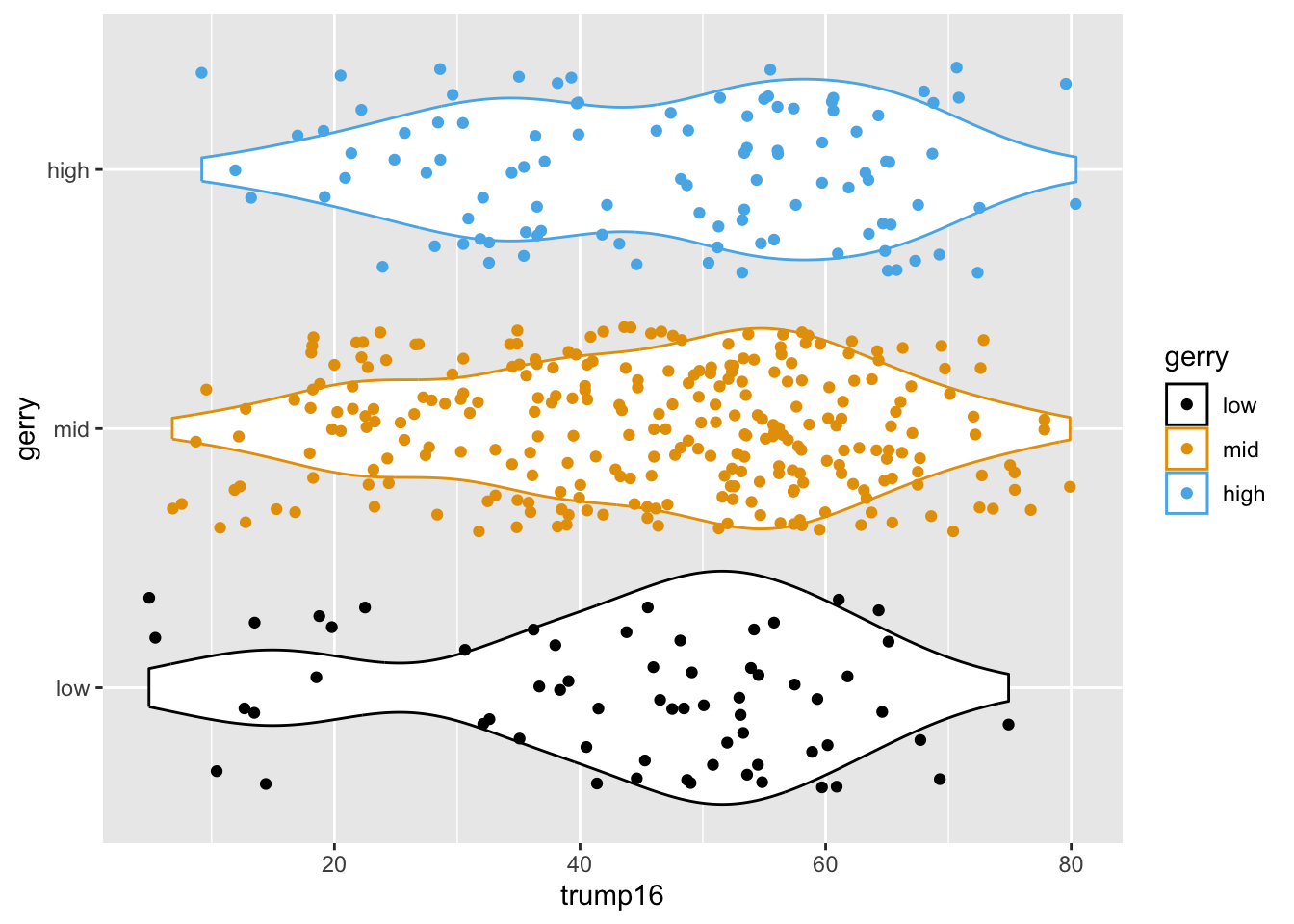
Remove legend