Exploring data II

Lecture 5

John Zito

Duke University
STA 199 Spring 2026

2026-01-28

Warm-up

While you wait…

Prepare for today’s application exercise: ae-05-gerrymander-explore-II

Go to your ae project in RStudio.
Make sure all of your changes up to this point are committed and pushed, i.e., there’s nothing left in your Git pane.
Click Pull to get today’s application exercise file: ae-05-gerrymander-explore-II.qmd.
Wait till the you’re prompted to work on the application exercise during class before editing the file.

Reminder: HW guidelines

Plots should include an informative title, axes and legends should have human-readable labels, and careful consideration should be given to aesthetic choices.
Code should follow the tidyverse style (style.tidyverse.org) Particularly,
- space before and line breaks after each + when building a ggplot
- space before and line breaks after each |> in a data transformation pipeline
- code should be properly indented
- spaces around = signs and spaces after commas
Proofread your rendered PDF before submission! We cannot give you points for stuff we cannot see, so make sure your code and output is not running off the page. Use line breaks.
At least three commits with meaningful commit messages.

Code style and readability

Whydowecareaboutthestyleandreadabilityofyourcode? \(\rightarrow\) Why do we care about the style and readability of your code?

Je voudrais un cafe \(\rightarrow\) Je voudrais un café

Monday takeaways

What data viz should I use?

After a while this is more art than science, but you can narrow down the options based on the number and type of variables:

Variable combo	Options
1 numerical	histogram, density, box plot
1 categorical	bar chart, ~~pie chart~~
2 numerical	scatterplot
numerical/categorical	side-by-side box or violin plots, stacked densities or histograms
2 categorical	stacked bar plot (today)

For three or more variables, the human mind is limited, and you have to start getting creative (play with color, texture, etc).

Pics are nice, but what are the numbers?

gerrymander |>
  summarize(
    gimme_my_mean = mean(trump16),
    gimme_my_median = median(trump16)
  )

summarize creates a new data frame that stores the summaries;
You can compute as many summaries as you want;
To the left of the equal signs are your choice of column names in the new data frame you are creating. You can type whatever you want here (within reason);
To the right of the equal signs is R code that computes the summaries. You must use the correct command names (case sensitive): mean, median, quantile, sd, var, etc;
If you want to learn what these do, read the documentation (eg ?quantile).

AE 4 speed run

Packages

For the data: usdata

library(usdata)

For the analysis: tidyverse and ggthemes

library(tidyverse)
library(ggthemes)

`gerrymander`

glimpse(gerrymander)

Rows: 435
Columns: 12
$ district   <chr> "AK-AL", "AL-01", "AL-02", "AL-03", "AL-04", "AL-05", "AL-0…
$ last_name  <chr> "Young", "Byrne", "Roby", "Rogers", "Aderholt", "Brooks", "…
$ first_name <chr> "Don", "Bradley", "Martha", "Mike D.", "Rob", "Mo", "Gary",…
$ party16    <chr> "R", "R", "R", "R", "R", "R", "R", "D", "R", "R", "R", "R",…
$ clinton16  <dbl> 37.6, 34.1, 33.0, 32.3, 17.4, 31.3, 26.1, 69.8, 30.2, 41.7,…
$ trump16    <dbl> 52.8, 63.5, 64.9, 65.3, 80.4, 64.7, 70.8, 28.6, 65.0, 52.4,…
$ dem16      <dbl> 0, 0, 0, 0, 0, 0, 0, 1, 0, 0, 0, 0, 1, 0, 1, 0, 0, 0, 1, 0,…
$ state      <chr> "AK", "AL", "AL", "AL", "AL", "AL", "AL", "AL", "AR", "AR",…
$ party18    <chr> "R", "R", "R", "R", "R", "R", "R", "D", "R", "R", "R", "R",…
$ dem18      <dbl> 0, 0, 0, 0, 0, 0, 0, 1, 0, 0, 0, 0, 1, 1, 1, 0, 0, 0, 1, 0,…
$ flip18     <dbl> 0, 0, 0, 0, 0, 0, 0, 0, 0, 0, 0, 0, 0, 1, 0, 0, 0, 0, 0, 0,…
$ gerry      <fct> mid, high, high, high, high, high, high, high, mid, mid, mi…

Research question

Is a Congressional District more likely to have high prevalence of gerrymandering if a Democrat was able to flip the seat in the 2018 election? Support your answer with a visualization as well as summary statistics.

Step 1

ggplot(gerrymander)

Step 2

ggplot(gerrymander, aes(x = flip18))

Step 3

ggplot(gerrymander, aes(x = flip18)) +
  geom_bar()

Step 4

ggplot(gerrymander, aes(x = flip18, fill = gerry)) +
  geom_bar()

Step 5a

ggplot(gerrymander, aes(x = flip18, fill = gerry)) +
  geom_bar(position = "dodge")

Step 5b

ggplot(gerrymander, aes(x = flip18, fill = gerry)) +
  geom_bar(position = "fill")

What’s the answer?

Is a Congressional District more likely to have high prevalence of gerrymandering if a Democrat was able to flip the seat in the 2018 election?

ggplot(gerrymander, aes(x = flip18, fill = gerry)) +
  geom_bar(position = "fill")

What are the actual numbers?

Is a Congressional District more likely to have high prevalence of gerrymandering if a Democrat was able to flip the seat in the 2018 election?

gerrymander |>
  count(flip18, gerry) |>
  group_by(flip18) |>
  mutate(prop = n / sum(n))

# A tibble: 8 × 4
# Groups:   flip18 [3]
  flip18 gerry     n  prop
   <dbl> <fct> <int> <dbl>
1     -1 low       2 0.4  
2     -1 mid       3 0.6  
3      0 low      52 0.133
4      0 mid     242 0.617
5      0 high     98 0.25 
6      1 low       8 0.211
7      1 mid      25 0.658
8      1 high      5 0.132

Step 1

gerrymander

# A tibble: 435 × 12
   district last_name first_name party16 clinton16 trump16 dem16 state party18
   <chr>    <chr>     <chr>      <chr>       <dbl>   <dbl> <dbl> <chr> <chr>  
 1 AK-AL    Young     Don        R            37.6    52.8     0 AK    R      
 2 AL-01    Byrne     Bradley    R            34.1    63.5     0 AL    R      
 3 AL-02    Roby      Martha     R            33      64.9     0 AL    R      
 4 AL-03    Rogers    Mike D.    R            32.3    65.3     0 AL    R      
 5 AL-04    Aderholt  Rob        R            17.4    80.4     0 AL    R      
 6 AL-05    Brooks    Mo         R            31.3    64.7     0 AL    R      
 7 AL-06    Palmer    Gary       R            26.1    70.8     0 AL    R      
 8 AL-07    Sewell    Terri      D            69.8    28.6     1 AL    D      
 9 AR-01    Crawford  Rick       R            30.2    65       0 AR    R      
10 AR-02    Hill      French     R            41.7    52.4     0 AR    R      
# ℹ 425 more rows
# ℹ 3 more variables: dem18 <dbl>, flip18 <dbl>, gerry <fct>

Step 2

gerrymander |>
  count(flip18, gerry)

# A tibble: 8 × 3
  flip18 gerry     n
   <dbl> <fct> <int>
1     -1 low       2
2     -1 mid       3
3      0 low      52
4      0 mid     242
5      0 high     98
6      1 low       8
7      1 mid      25
8      1 high      5

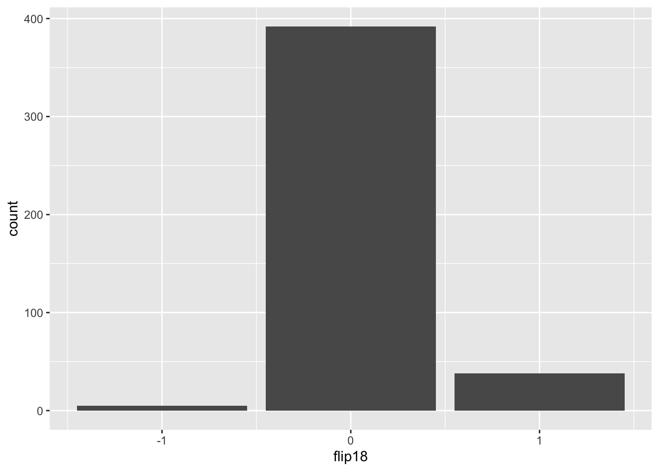
Recall

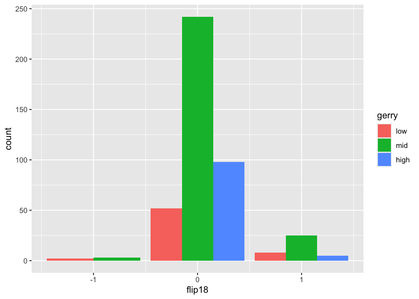
The heights of these bars are the counts in the table:

ggplot(gerrymander, aes(x = flip18, fill = gerry)) +
  geom_bar(position = "dodge")

Step 3

gerrymander |>
  count(flip18, gerry) |>
  group_by(flip18)

# A tibble: 8 × 3
# Groups:   flip18 [3]
  flip18 gerry     n
   <dbl> <fct> <int>
1     -1 low       2
2     -1 mid       3
3      0 low      52
4      0 mid     242
5      0 high     98
6      1 low       8
7      1 mid      25
8      1 high      5

Step 4

gerrymander |>
  count(flip18, gerry) |>
  group_by(flip18) |>
  mutate(prop = n / sum(n))

# A tibble: 8 × 4
# Groups:   flip18 [3]
  flip18 gerry     n  prop
   <dbl> <fct> <int> <dbl>
1     -1 low       2 0.4  
2     -1 mid       3 0.6  
3      0 low      52 0.133
4      0 mid     242 0.617
5      0 high     98 0.25 
6      1 low       8 0.211
7      1 mid      25 0.658
8      1 high      5 0.132

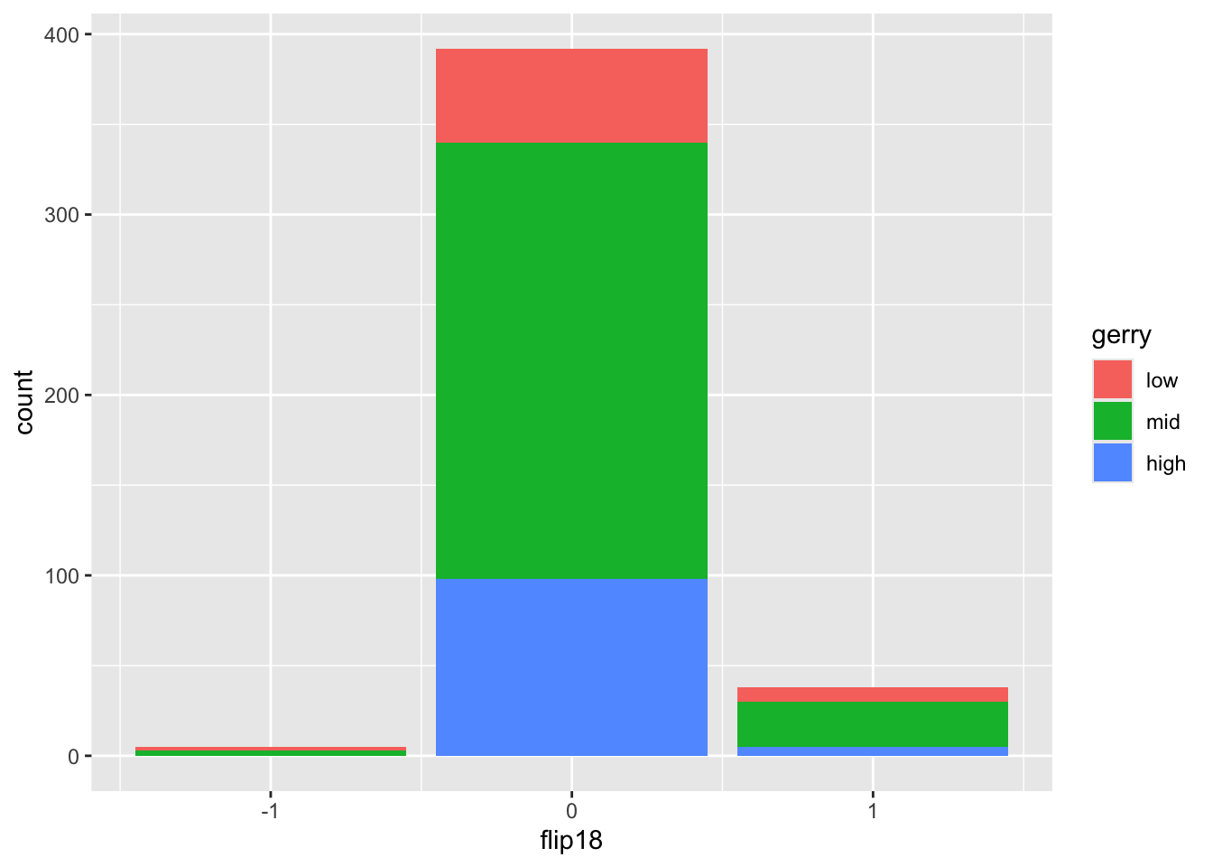
The Full Monty

Is a Congressional District more likely to have high prevalence of gerrymandering if a Democrat flipped the seat in the 2018 election? (flip18 = 1: Democrat flipped the seat, 0: No flip, -1: Republican flipped the seat.)

ggplot(
  gerrymander, 
  aes(x = flip18, fill = gerry)
  ) +
  geom_bar(position = "fill")

gerrymander |>
  count(flip18, gerry) |>
  group_by(flip18) |>
  mutate(prop = n / sum(n))

# A tibble: 8 × 4
# Groups:   flip18 [3]
  flip18 gerry     n  prop
   <dbl> <fct> <int> <dbl>
1     -1 low       2 0.4  
2     -1 mid       3 0.6  
3      0 low      52 0.133
4      0 mid     242 0.617
5      0 high     98 0.25 
6      1 low       8 0.211
7      1 mid      25 0.658
8      1 high      5 0.132

New commands

count creates a new data frame that tallies up the number of rows that fall into each bin;
group_by silently groups the rows according to bin, and all subsequent operations are done within group;
mutate either adds new columns that aren’t already there, or modifies existing columns.
- we used it to add a prop column that wasn’t there before;
- because the table of counts is grouped, the proportions were computed within each level of flip18.

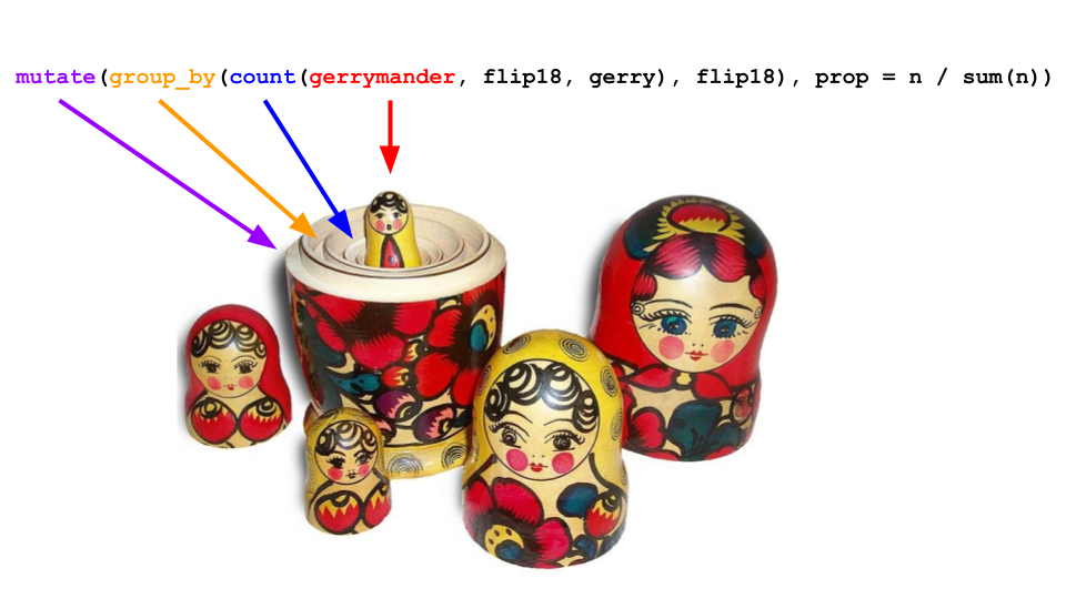
That pesky pipe

We teach you to do this

gerrymander |>
  count(flip18, gerry) |>
  group_by(flip18) |>
  mutate(prop = n / sum(n))

# A tibble: 8 × 4
# Groups:   flip18 [3]
  flip18 gerry     n  prop
   <dbl> <fct> <int> <dbl>
1     -1 low       2 0.4  
2     -1 mid       3 0.6  
3      0 low      52 0.133
4      0 mid     242 0.617
5      0 high     98 0.25 
6      1 low       8 0.211
7      1 mid      25 0.658
8      1 high      5 0.132

You could do this instead

Technically equivalent. Gives the same result. Super hard to read:

mutate(group_by(count(gerrymander, flip18, gerry), flip18), prop = n / sum(n))

# A tibble: 8 × 4
# Groups:   flip18 [3]
  flip18 gerry     n  prop
   <dbl> <fct> <int> <dbl>
1     -1 low       2 0.4  
2     -1 mid       3 0.6  
3      0 low      52 0.133
4      0 mid     242 0.617
5      0 high     98 0.25 
6      1 low       8 0.211
7      1 mid      25 0.658
8      1 high      5 0.132

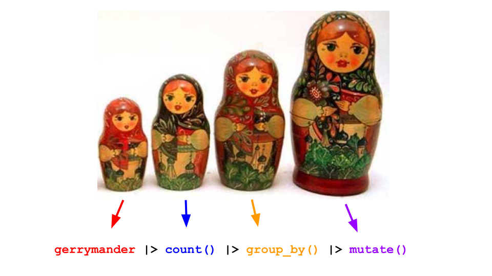
Without the pipe

With the pipe

In this class, you will…

Build cakes (ggplot)

Stack dolls (pipe |>)

Master these constructs, and everything will be coming up roses!

(Secrets of the temple)

For all you CS people and prospective stats majors:

There is more to R than ggplot and |>;
It’s a proper programming language like Python, C++, Java, etc;
- control flow, data structures, OOP, all that good stuff;
In STAWANANA, we suppress all that and teach you a very specific dialect of R called the tidyverse;
Keep studying stats, and we show you how to use the whole language to do statistical computing, not just data science.

Drilling down:
`group_by()`,
`summarize()`,
`count()`

What does `group_by()` do?

What does group_by() do in the following pipeline?

gerrymander |>
  count(flip18, gerry) |>
  group_by(flip18) |>
  mutate(prop = n / sum(n))

# A tibble: 8 × 4
# Groups:   flip18 [3]
  flip18 gerry     n  prop
   <dbl> <fct> <int> <dbl>
1     -1 low       2 0.4  
2     -1 mid       3 0.6  
3      0 low      52 0.133
4      0 mid     242 0.617
5      0 high     98 0.25 
6      1 low       8 0.211
7      1 mid      25 0.658
8      1 high      5 0.132

What does `group_by()` do?

What does group_by() do in the following pipeline?

gerrymander |>
  count(flip18, gerry) |>
  #group_by(flip18) |>
  mutate(prop = n / sum(n))

# A tibble: 8 × 4
  flip18 gerry     n    prop
   <dbl> <fct> <int>   <dbl>
1     -1 low       2 0.00460
2     -1 mid       3 0.00690
3      0 low      52 0.120  
4      0 mid     242 0.556  
5      0 high     98 0.225  
6      1 low       8 0.0184 
7      1 mid      25 0.0575 
8      1 high      5 0.0115

Let’s simplify!

What does group_by() do in the following pipeline?

gerrymander |>
  group_by(state) |>
  summarize(mean_trump16 = mean(trump16))

# A tibble: 50 × 2
   state mean_trump16
   <chr>        <dbl>
 1 AK            52.8
 2 AL            62.6
 3 AR            60.9
 4 AZ            46.9
 5 CA            31.7
 6 CO            43.6
 7 CT            41.0
 8 DE            41.9
 9 FL            47.9
10 GA            51.3
# ℹ 40 more rows

Let’s simplify!

What does group_by() do in the following pipeline?

gerrymander |>
  #group_by(state) |>
  summarize(mean_trump16 = mean(trump16))

# A tibble: 1 × 1
  mean_trump16
         <dbl>
1         45.9

`group_by()`

it converts a data frame to a grouped data frame, where subsequent operations are performed once per group
ungroup() removes grouping

gerrymander |>
  group_by(state)

# A tibble: 435 × 12
# Groups:   state [50]
   district last_name first_name party16 clinton16 trump16 dem16 state party18
   <chr>    <chr>     <chr>      <chr>       <dbl>   <dbl> <dbl> <chr> <chr>  
 1 AK-AL    Young     Don        R            37.6    52.8     0 AK    R      
 2 AL-01    Byrne     Bradley    R            34.1    63.5     0 AL    R      
 3 AL-02    Roby      Martha     R            33      64.9     0 AL    R      
 4 AL-03    Rogers    Mike D.    R            32.3    65.3     0 AL    R      
 5 AL-04    Aderholt  Rob        R            17.4    80.4     0 AL    R      
 6 AL-05    Brooks    Mo         R            31.3    64.7     0 AL    R      
 7 AL-06    Palmer    Gary       R            26.1    70.8     0 AL    R      
 8 AL-07    Sewell    Terri      D            69.8    28.6     1 AL    D      
 9 AR-01    Crawford  Rick       R            30.2    65       0 AR    R      
10 AR-02    Hill      French     R            41.7    52.4     0 AR    R      
# ℹ 425 more rows
# ℹ 3 more variables: dem18 <dbl>, flip18 <dbl>, gerry <fct>

`group_by()`

it converts a data frame to a grouped data frame, where subsequent operations are performed once per group
ungroup() removes grouping

gerrymander |>
  group_by(state) |>
  ungroup()

# A tibble: 435 × 12
   district last_name first_name party16 clinton16 trump16 dem16 state party18
   <chr>    <chr>     <chr>      <chr>       <dbl>   <dbl> <dbl> <chr> <chr>  
 1 AK-AL    Young     Don        R            37.6    52.8     0 AK    R      
 2 AL-01    Byrne     Bradley    R            34.1    63.5     0 AL    R      
 3 AL-02    Roby      Martha     R            33      64.9     0 AL    R      
 4 AL-03    Rogers    Mike D.    R            32.3    65.3     0 AL    R      
 5 AL-04    Aderholt  Rob        R            17.4    80.4     0 AL    R      
 6 AL-05    Brooks    Mo         R            31.3    64.7     0 AL    R      
 7 AL-06    Palmer    Gary       R            26.1    70.8     0 AL    R      
 8 AL-07    Sewell    Terri      D            69.8    28.6     1 AL    D      
 9 AR-01    Crawford  Rick       R            30.2    65       0 AR    R      
10 AR-02    Hill      French     R            41.7    52.4     0 AR    R      
# ℹ 425 more rows
# ℹ 3 more variables: dem18 <dbl>, flip18 <dbl>, gerry <fct>

`group_by() |> summarize()`

A common pipeline is group_by() and then summarize() to calculate summary statistics for each group:

gerrymander |>
  group_by(state) |>
  summarize(
    mean_trump16 = mean(trump16),
    median_trump16 = median(trump16)
  )

# A tibble: 50 × 3
   state mean_trump16 median_trump16
   <chr>        <dbl>          <dbl>
 1 AK            52.8           52.8
 2 AL            62.6           64.9
 3 AR            60.9           63.0
 4 AZ            46.9           47.7
 5 CA            31.7           28.4
 6 CO            43.6           41.3
 7 CT            41.0           40.4
 8 DE            41.9           41.9
 9 FL            47.9           49.6
10 GA            51.3           56.6
# ℹ 40 more rows

`group_by() |> summarize()`

This pipeline can also be used to count number of observations for each group:

gerrymander |>
  group_by(state) |>
  summarize(n = n())

# A tibble: 50 × 2
   state     n
   <chr> <int>
 1 AK        1
 2 AL        7
 3 AR        4
 4 AZ        9
 5 CA       53
 6 CO        7
 7 CT        5
 8 DE        1
 9 FL       27
10 GA       14
# ℹ 40 more rows

`summarize()`

... |>
  summarize(
    name_of_summary_statistic = summary_function(variable)
  )

name_of_summary_statistic: Anything you want to call it!
- Recommendation: Keep it short and evocative
summary_function():
- n(): number of observations
- mean(): mean
- median(): median
- …

Spot the difference

What’s the difference between the following two pipelines?

gerrymander |>
  group_by(state) |>
  summarize(n = n())

# A tibble: 50 × 2
   state     n
   <chr> <int>
 1 AK        1
 2 AL        7
 3 AR        4
 4 AZ        9
 5 CA       53
 6 CO        7
 7 CT        5
 8 DE        1
 9 FL       27
10 GA       14
# ℹ 40 more rows

gerrymander |>
  count(state)

# A tibble: 50 × 2
   state     n
   <chr> <int>
 1 AK        1
 2 AL        7
 3 AR        4
 4 AZ        9
 5 CA       53
 6 CO        7
 7 CT        5
 8 DE        1
 9 FL       27
10 GA       14
# ℹ 40 more rows

`count()`

... |>
  count(variable)

... |>
  count(variable1, variable2)

Count the number of observations in each level of variable(s)
Place the counts in a variable called n

`count()` and `sort`

What does the following pipeline do? Rewrite it with count() instead.

gerrymander |>
  group_by(state) |>
  summarize(n = n()) |>
  arrange(desc(n))

# A tibble: 50 × 2
   state     n
   <chr> <int>
 1 CA       53
 2 TX       36
 3 FL       27
 4 NY       27
 5 IL       18
 6 PA       18
 7 OH       16
 8 GA       14
 9 MI       14
10 NC       13
# ℹ 40 more rows

`count()` and `sort`

What does the following pipeline do? Rewrite it with count() instead.

gerrymander |>
  count(state) |>
  arrange(desc(n))

# A tibble: 50 × 2
   state     n
   <chr> <int>
 1 CA       53
 2 TX       36
 3 FL       27
 4 NY       27
 5 IL       18
 6 PA       18
 7 OH       16
 8 GA       14
 9 MI       14
10 NC       13
# ℹ 40 more rows

`count()` and `sort`

What does the following pipeline do? Rewrite it with count() instead.

gerrymander |>
  count(state, sort = TRUE)

# A tibble: 50 × 2
   state     n
   <chr> <int>
 1 CA       53
 2 TX       36
 3 FL       27
 4 NY       27
 5 IL       18
 6 PA       18
 7 OH       16
 8 GA       14
 9 MI       14
10 NC       13
# ℹ 40 more rows

`mutate()`

Flip the question

Note

Is a Congressional District more likely to have high prevalence of gerrymandering if a Democrat was able to flip the seat in the 2018 election?

vs.

Note

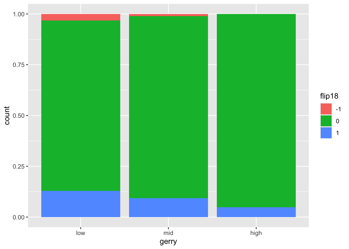
Is a Congressional District more likely to be flipped to a Democratic seat if it has high prevalence of gerrymandering or low prevalence of gerrymandering?

Flipping vs. gerrymandering prevalence

The following code should produce a visualization that answers the question “Is a Congressional District more likely to be flipped to a Democratic seat if it has high prevalence of gerrymandering or low prevalence of gerrymandering?” However, it produces a warning and an unexpected plot. What’s going on?

ggplot(
  gerrymander, 
  aes(x = gerry, fill = flip18)
  ) +
  geom_bar(position = "fill")

Warning: The following aesthetics were dropped during statistical transformation: fill.
ℹ This can happen when ggplot fails to infer the correct grouping structure in
  the data.
ℹ Did you forget to specify a `group` aesthetic or to convert a numerical
  variable into a factor?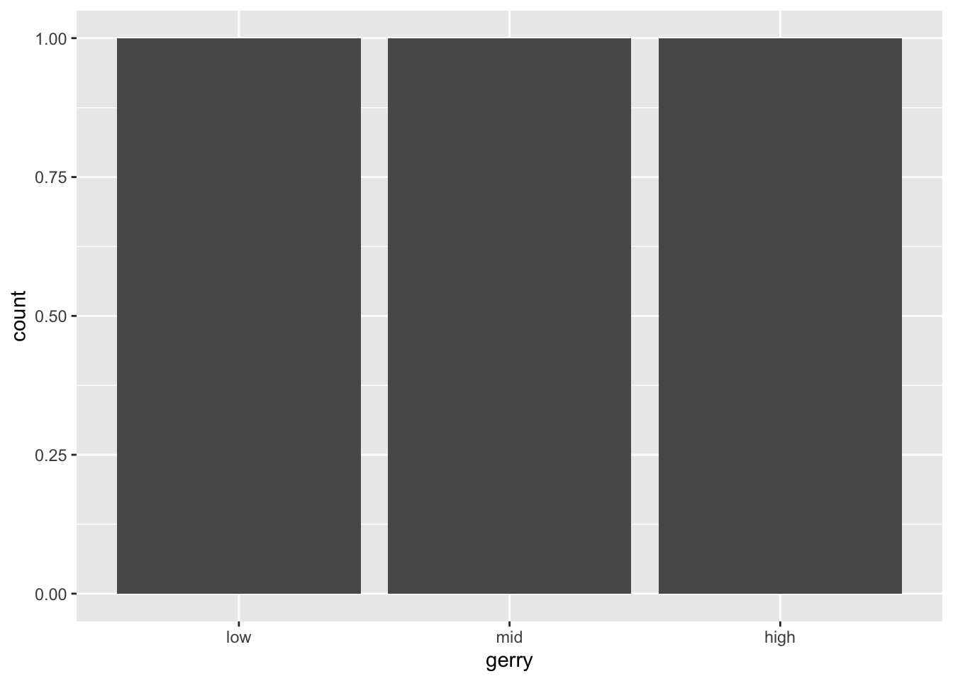

Another glimpse at `gerrymander`

glimpse(gerrymander)

Rows: 435
Columns: 12
$ district   <chr> "AK-AL", "AL-01", "AL-02", "AL-03", "AL-04", "AL-05", "AL-0…
$ last_name  <chr> "Young", "Byrne", "Roby", "Rogers", "Aderholt", "Brooks", "…
$ first_name <chr> "Don", "Bradley", "Martha", "Mike D.", "Rob", "Mo", "Gary",…
$ party16    <chr> "R", "R", "R", "R", "R", "R", "R", "D", "R", "R", "R", "R",…
$ clinton16  <dbl> 37.6, 34.1, 33.0, 32.3, 17.4, 31.3, 26.1, 69.8, 30.2, 41.7,…
$ trump16    <dbl> 52.8, 63.5, 64.9, 65.3, 80.4, 64.7, 70.8, 28.6, 65.0, 52.4,…
$ dem16      <dbl> 0, 0, 0, 0, 0, 0, 0, 1, 0, 0, 0, 0, 1, 0, 1, 0, 0, 0, 1, 0,…
$ state      <chr> "AK", "AL", "AL", "AL", "AL", "AL", "AL", "AL", "AR", "AR",…
$ party18    <chr> "R", "R", "R", "R", "R", "R", "R", "D", "R", "R", "R", "R",…
$ dem18      <dbl> 0, 0, 0, 0, 0, 0, 0, 1, 0, 0, 0, 0, 1, 1, 1, 0, 0, 0, 1, 0,…
$ flip18     <dbl> 0, 0, 0, 0, 0, 0, 0, 0, 0, 0, 0, 0, 0, 1, 0, 0, 0, 0, 0, 0,…
$ gerry      <fct> mid, high, high, high, high, high, high, high, mid, mid, mi…

`mutate()`

We want to use flip18 as a categorical variable
But it’s stored as a numeric
So we need to change its type first, before we can use it as a categorical variable
The mutate() function transforms (mutates) a data frame by creating a new column or updating an existing one

In this case, we want to use it to update an existing column, flip18.

`mutate()` in action

gerrymander |>
  mutate(flip18 = as_factor(flip18))

# A tibble: 435 × 12
   district last_name first_name party16 clinton16 trump16 dem16 state party18
   <chr>    <chr>     <chr>      <chr>       <dbl>   <dbl> <dbl> <chr> <chr>  
 1 AK-AL    Young     Don        R            37.6    52.8     0 AK    R      
 2 AL-01    Byrne     Bradley    R            34.1    63.5     0 AL    R      
 3 AL-02    Roby      Martha     R            33      64.9     0 AL    R      
 4 AL-03    Rogers    Mike D.    R            32.3    65.3     0 AL    R      
 5 AL-04    Aderholt  Rob        R            17.4    80.4     0 AL    R      
 6 AL-05    Brooks    Mo         R            31.3    64.7     0 AL    R      
 7 AL-06    Palmer    Gary       R            26.1    70.8     0 AL    R      
 8 AL-07    Sewell    Terri      D            69.8    28.6     1 AL    D      
 9 AR-01    Crawford  Rick       R            30.2    65       0 AR    R      
10 AR-02    Hill      French     R            41.7    52.4     0 AR    R      
# ℹ 425 more rows
# ℹ 3 more variables: dem18 <dbl>, flip18 <fct>, gerry <fct>

`mutate()` in action

gerrymander |>
  mutate(flip18 = as_factor(flip18)) |>
  relocate(flip18)

# A tibble: 435 × 12
   flip18 district last_name first_name party16 clinton16 trump16 dem16 state
   <fct>  <chr>    <chr>     <chr>      <chr>       <dbl>   <dbl> <dbl> <chr>
 1 0      AK-AL    Young     Don        R            37.6    52.8     0 AK   
 2 0      AL-01    Byrne     Bradley    R            34.1    63.5     0 AL   
 3 0      AL-02    Roby      Martha     R            33      64.9     0 AL   
 4 0      AL-03    Rogers    Mike D.    R            32.3    65.3     0 AL   
 5 0      AL-04    Aderholt  Rob        R            17.4    80.4     0 AL   
 6 0      AL-05    Brooks    Mo         R            31.3    64.7     0 AL   
 7 0      AL-06    Palmer    Gary       R            26.1    70.8     0 AL   
 8 0      AL-07    Sewell    Terri      D            69.8    28.6     1 AL   
 9 0      AR-01    Crawford  Rick       R            30.2    65       0 AR   
10 0      AR-02    Hill      French     R            41.7    52.4     0 AR   
# ℹ 425 more rows
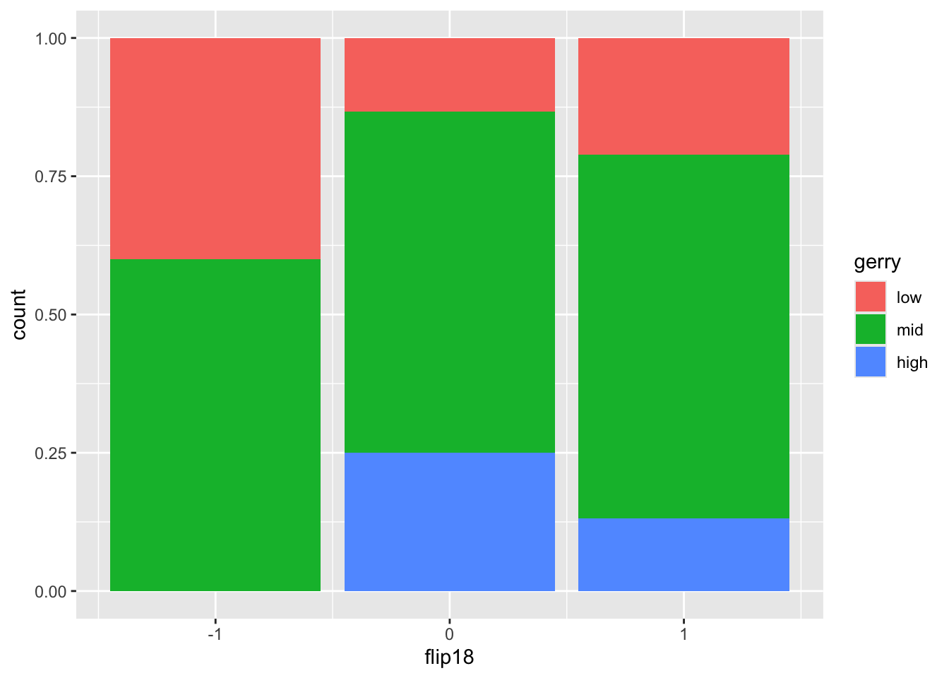
# ℹ 3 more variables: party18 <chr>, dem18 <dbl>, gerry <fct>

Revisit the plot

“Is a Congressional District more likely to be flipped to a Democratic seat if it has high prevalence of gerrymandering or low prevalence of gerrymandering?”

gerrymander |>
  mutate(flip18 = as_factor(flip18)) |>
  ggplot(aes(x = gerry, fill = flip18)) +
  geom_bar(position = "fill")

`mutate()` and overwrite

You can overwrite an existing variable with mutate():

gerrymander |>
  mutate(flip18 = as_factor(flip18)) |>
  select(district, flip18)

# A tibble: 435 × 2
   district flip18
   <chr>    <fct> 
 1 AK-AL    0     
 2 AL-01    0     
 3 AL-02    0     
 4 AL-03    0     
 5 AL-04    0     
 6 AL-05    0     
 7 AL-06    0     
 8 AL-07    0     
 9 AR-01    0     
10 AR-02    0     
# ℹ 425 more rows

`mutate()` and `if_else()`

Use mutate() with if_else() to recode with an either/or logic:

If party16 is “D”, recode it as “Democrat”, otherwise recode it as “Republican”.

gerrymander |>
  mutate(party16_expanded = if_else(party16 == "D", "Democrat", "Republican")) |>
  select(district, party16, party16_expanded)

# A tibble: 435 × 3
   district party16 party16_expanded
   <chr>    <chr>   <chr>           
 1 AK-AL    R       Republican      
 2 AL-01    R       Republican      
 3 AL-02    R       Republican      
 4 AL-03    R       Republican      
 5 AL-04    R       Republican      
 6 AL-05    R       Republican      
 7 AL-06    R       Republican      
 8 AL-07    D       Democrat        
 9 AR-01    R       Republican      
10 AR-02    R       Republican      
# ℹ 425 more rows

`mutate()` and `case_when()`

Use mutate() with case_when() to recode with a more complex logic:

If flip18 is 1, recode it as “Democrat flipped”, if flip18 is 0, recode it as “No flip”, and if flip18 is -1, recode it as “Republican flipped”.

gerrymander |>
  mutate(
    flip18_expanded = case_when(
      flip18 == 1 ~ "Democrat flipped",
      flip18 == 0 ~ "No flip",
      flip18 == -1 ~ "Republican flipped"
    )
  ) |>
  select(district, flip18, flip18_expanded) |>
  group_by(flip18) |> # group by flip type
  slice_head(n = 1) # show top row per group

# A tibble: 3 × 3
# Groups:   flip18 [3]
  district flip18 flip18_expanded   
  <chr>     <dbl> <chr>             
1 MN-01        -1 Republican flipped
2 AK-AL         0 No flip           
3 AZ-02         1 Democrat flipped

`mutate()` and store

If you want to keep your changes, you need to store the data frame after mutate():

gerrymander |>
  mutate(
    p16 = if_else(party16 == "D", "Dem", "Rep")
  ) |>
  select(district, p16) |>
  slice_head(n = 3) # show top 3 rows

# A tibble: 3 × 2
  district p16  
  <chr>    <chr>
1 AK-AL    Rep  
2 AL-01    Rep  
3 AL-02    Rep

gerrymander |>
  select(district, p16)

Error in `select()`:
! Can't select columns that don't exist.
✖ Column `p16` doesn't exist.

gerrymander <- gerrymander |>
  mutate(
    p16 = if_else(party16 == "D", "Dem", "Rep")
  ) |>
  select(district, p16)

gerrymander |>
  select(district, p16)  |>
  slice_head(n = 3) # show top 3 rows

# A tibble: 3 × 2
  district p16  
  <chr>    <chr>
1 AK-AL    Rep  
2 AL-01    Rep  
3 AL-02    Rep

Application exercise

ae-05-gerrymander-explore-II

Go to your ae project in RStudio.
If you haven’t yet done so, make sure all of your changes up to this point are committed and pushed, i.e., there’s nothing left in your Git pane.
If you haven’t yet done so, click Pull to get today’s application exercise file: ae-05-gerrymander-explore-II.qmd.
Work through the application exercise in class, and render, commit, and push your edits by the end of class.

Recap: aesthetic mappings

Local aesthetic mappings for a given geom
Global aesthetic mappings for all geoms

Exploring data II

Warm-up

While you wait…

Reminder: HW guidelines

Code style and readability

Monday takeaways

What data viz should I use?

Pics are nice, but what are the numbers?

AE 4 speed run

Packages

gerrymander

Research question

Step 1

Step 2

Step 3

Step 4

Step 5a

Step 5b

What’s the answer?

What are the actual numbers?

Step 1

Step 2

Recall

Step 3

Step 4

The Full Monty

New commands

That pesky pipe

We teach you to do this

You could do this instead

Without the pipe

With the pipe

In this class, you will…

(Secrets of the temple)

Drilling down: group_by(), summarize(), count()

What does group_by() do?

What does group_by() do?

Let’s simplify!

Let’s simplify!

group_by()

group_by()

group_by() |> summarize()

group_by() |> summarize()

summarize()

Spot the difference

count()

count() and sort

count() and sort

count() and sort

mutate()

Flip the question

Flipping vs. gerrymandering prevalence

Another glimpse at gerrymander

mutate()

mutate() in action

mutate() in action

Revisit the plot

mutate() and overwrite

mutate() and if_else()

mutate() and case_when()

mutate() and store

Application exercise

ae-05-gerrymander-explore-II

Recap: aesthetic mappings

`gerrymander`

Drilling down:
`group_by()`,
`summarize()`,
`count()`

What does `group_by()` do?

What does `group_by()` do?

`group_by()`

`group_by()`

`group_by() |> summarize()`

`group_by() |> summarize()`

`summarize()`

`count()`

`count()` and `sort`

`count()` and `sort`

`count()` and `sort`

`mutate()`

Another glimpse at `gerrymander`

`mutate()`

`mutate()` in action

`mutate()` in action

`mutate()` and overwrite

`mutate()` and `if_else()`

`mutate()` and `case_when()`

`mutate()` and store