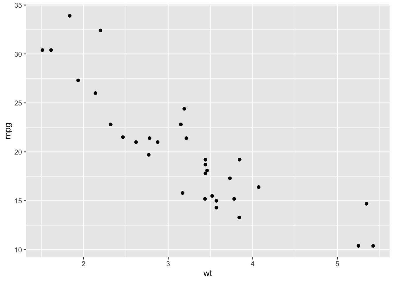
| mpg | wt |
|---|---|
| 21 | 2.62 |
| 21 | 2.875 |
| 22.8 | 2.32 |
| 21.4 | 3.215 |
| 18.7 | 3.44 |
| 18.1 | 3.46 |
| ... | ... |
The language of models
Lecture 15
2026-03-16
DataFest

- Sign up here!
- Teams of your choice explore a mystery dataset and blitz an analysis in two days;
- Starts Friday March 20 @ 5PM;
- Ends Sunday March 22 @ 5PM;
- Free food!
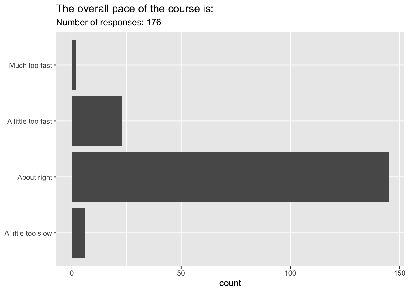
The overall pace of the course is…
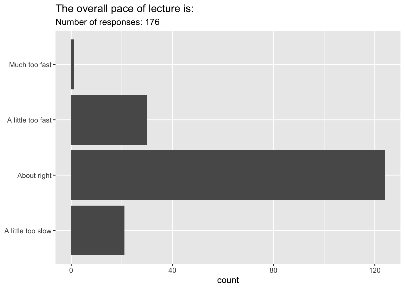
The overall pace of lecture is…
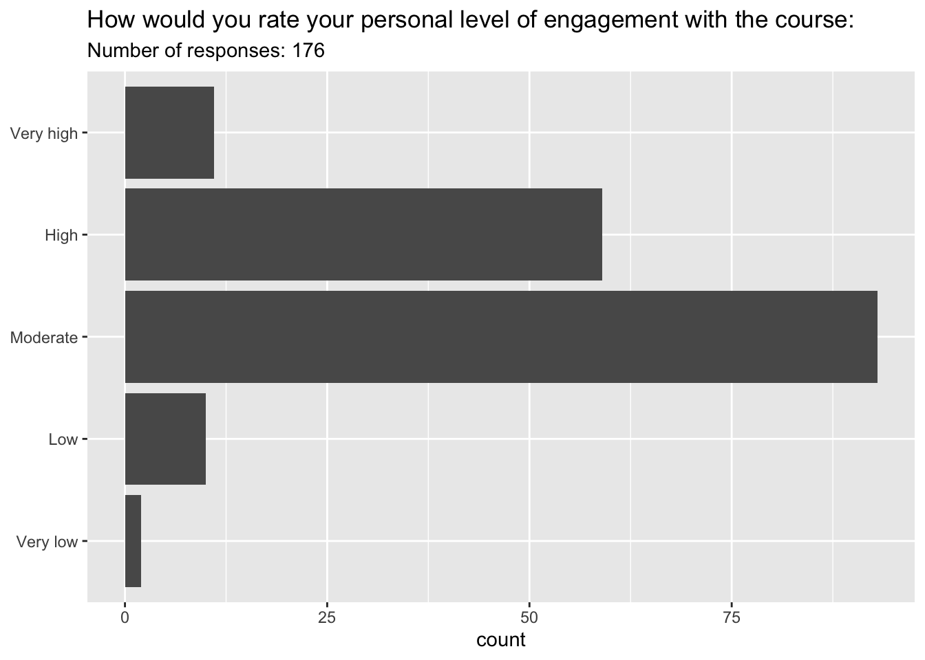
How would you rate your personal level of engagement with the course?
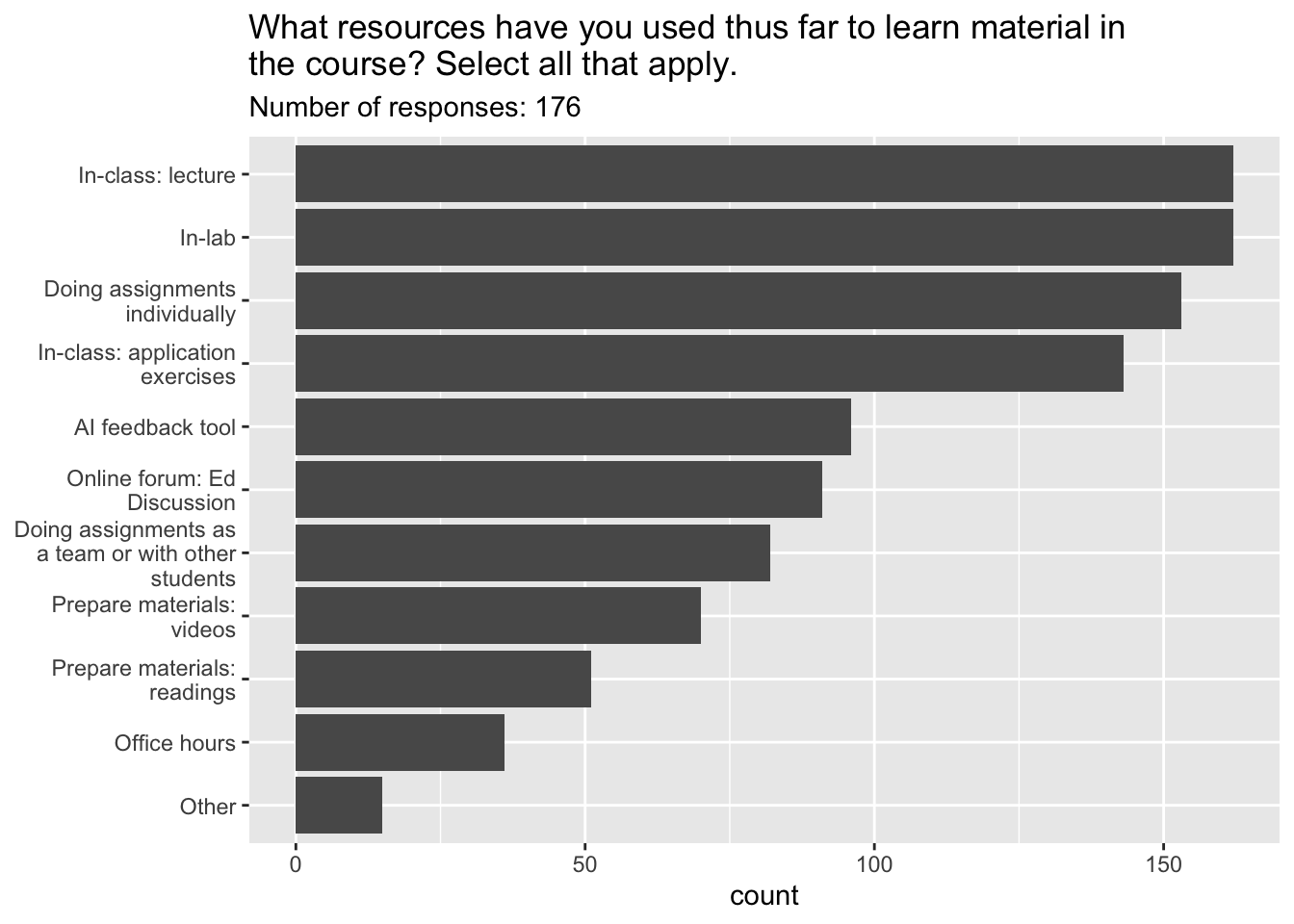
What resources have you used thus far to learn material in the course?
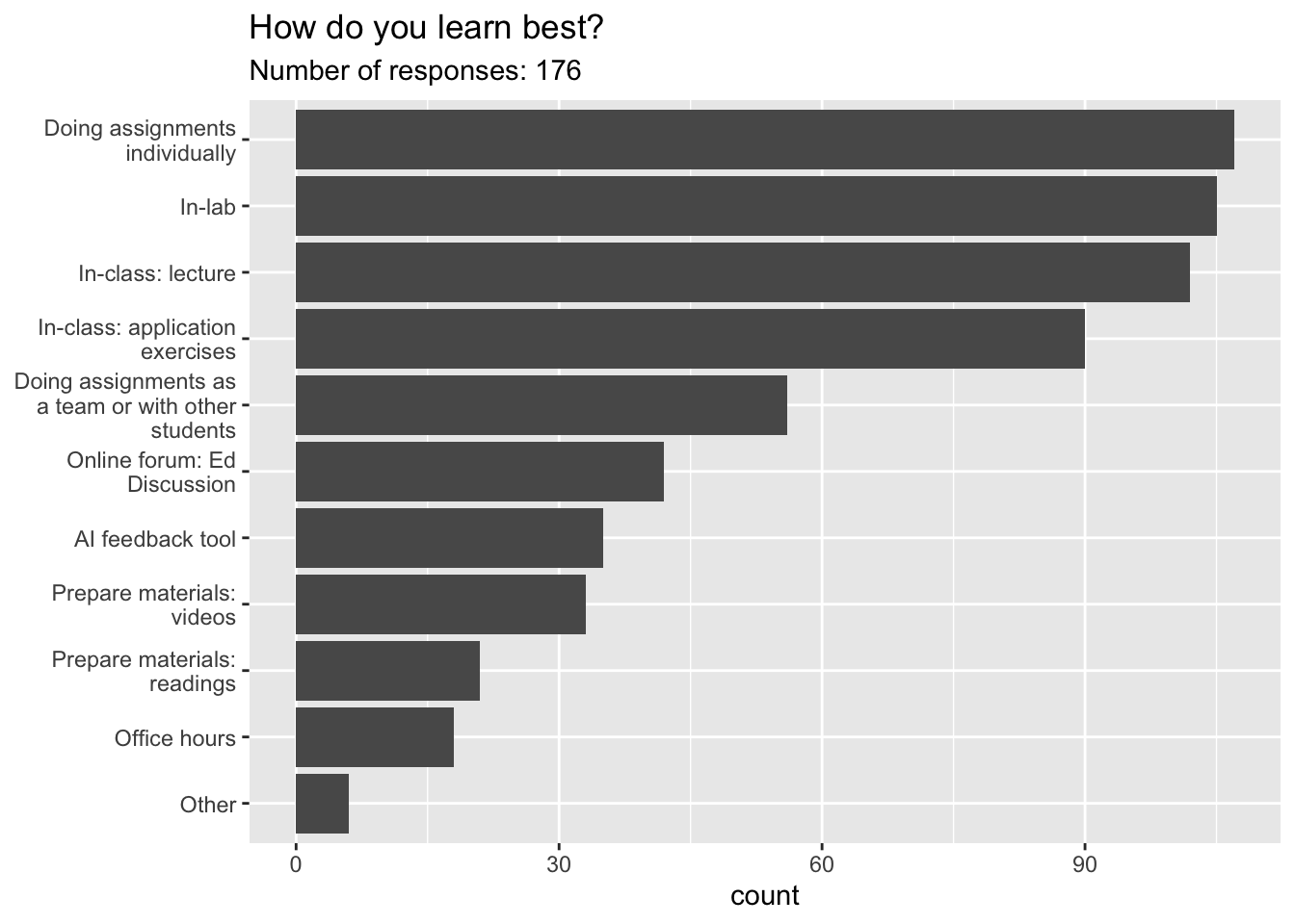
How have you learned the best so far in the class?
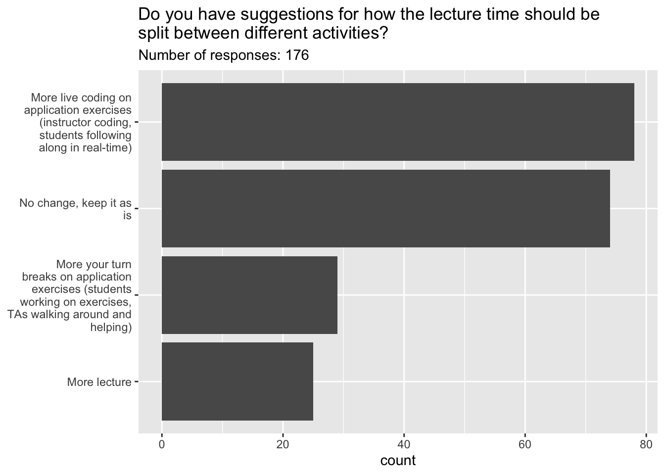
Do you have suggestions for how the lecture time should be split between different activities?
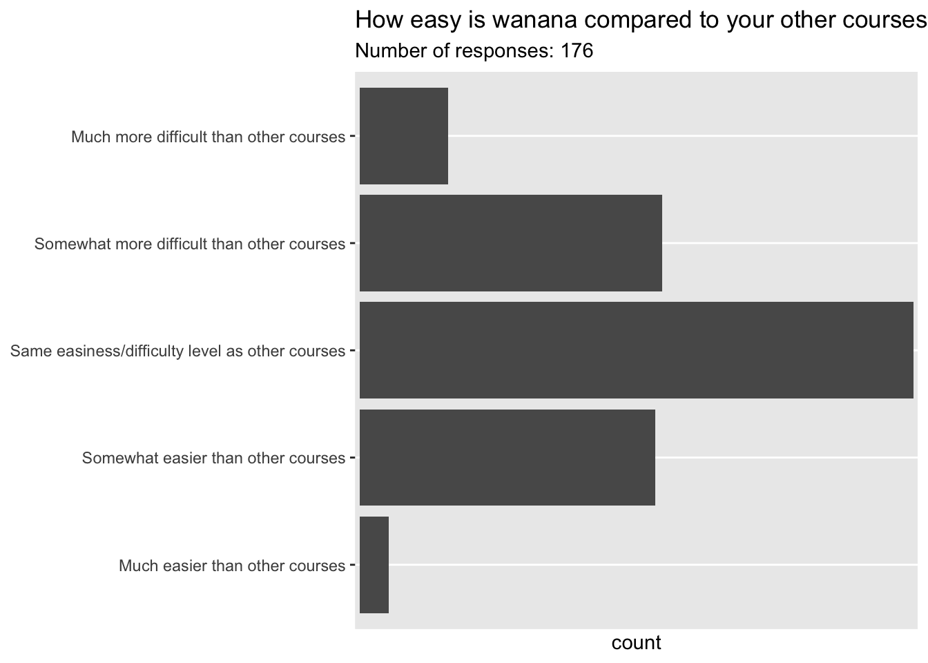
How easy is this course compared to your other courses?
Semi or garage?
i love how Tesla thinks the wall in my garage is a semi. 😅
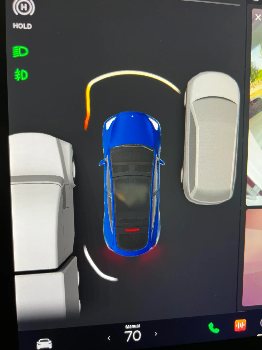
Semi or garage?
New owner here. Just parked in my garage. Tesla thinks I crashed onto a semi.

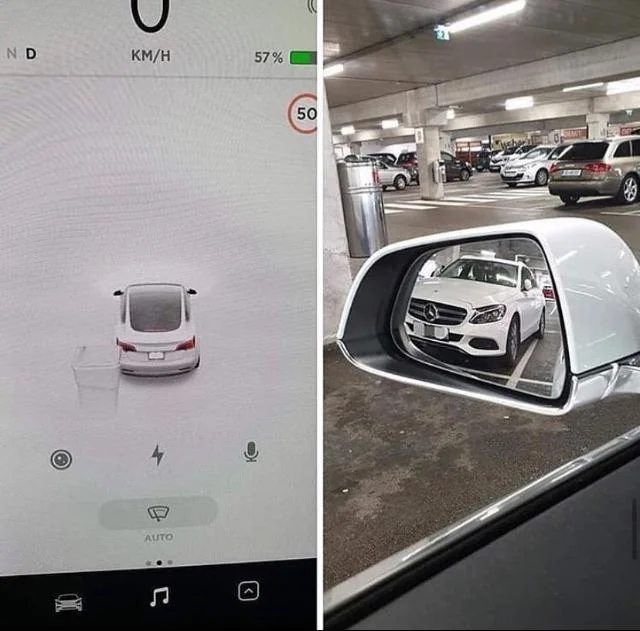
Car or trash?
Tesla calls Mercedes trash
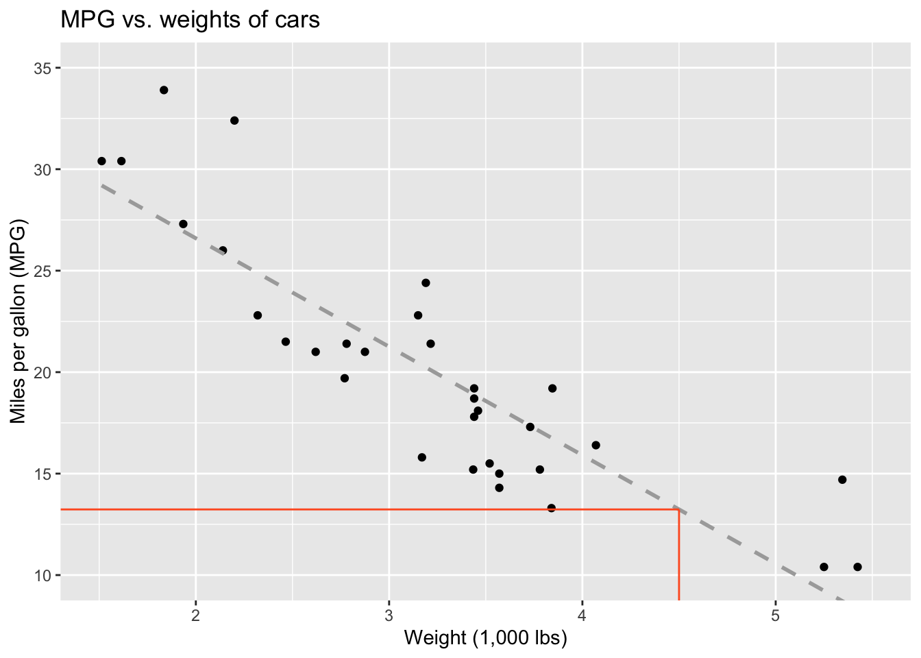
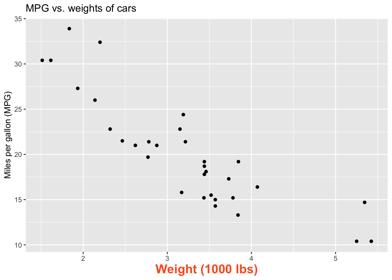
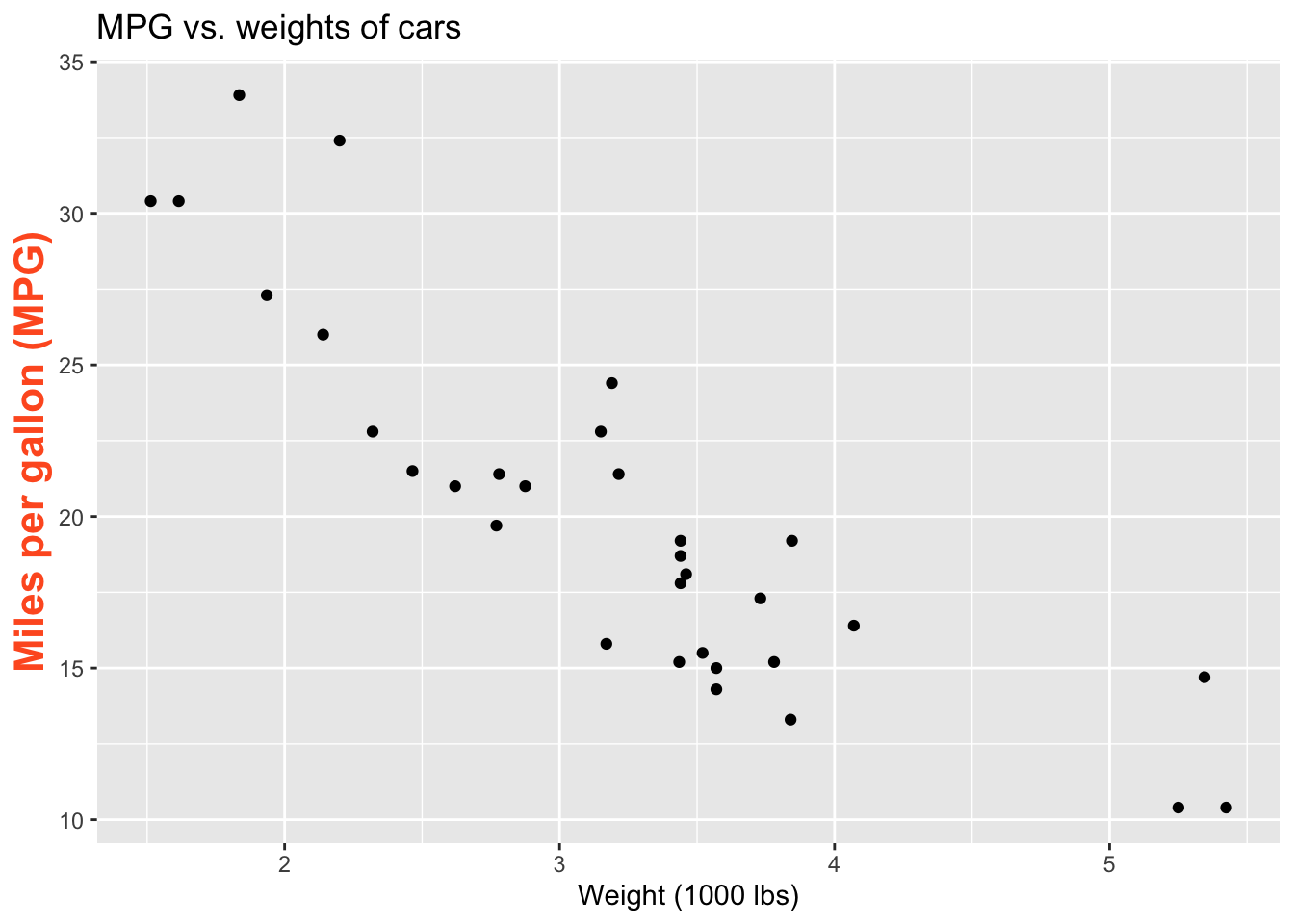
Modeling cars
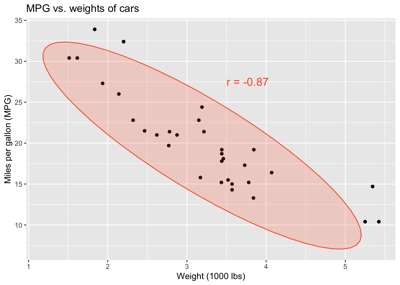
- What is the relationship between cars’ weights and their mileage?
- What is your best guess for a car’s MPG that weighs 4,500 pounds?
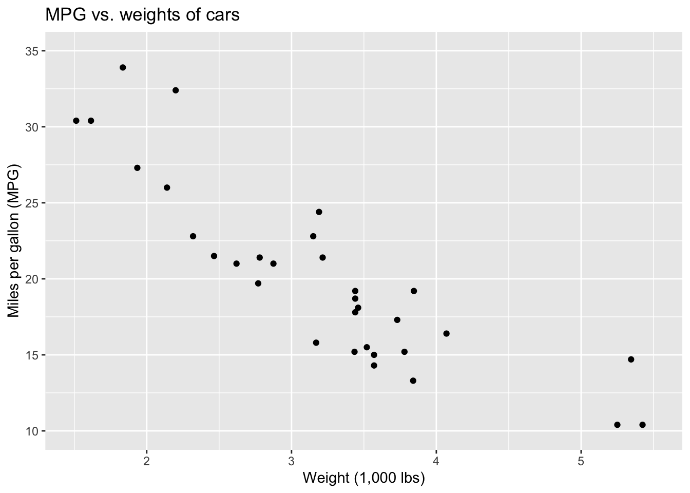
Modelling cars
Describe: What is the relationship between cars’ weights and their mileage?
Modelling cars
Predict: What is your best guess for a car’s MPG that weighs 4,500 pounds?
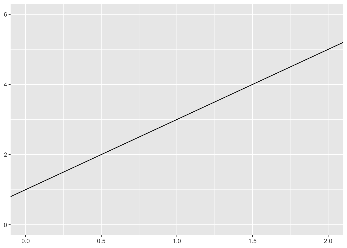
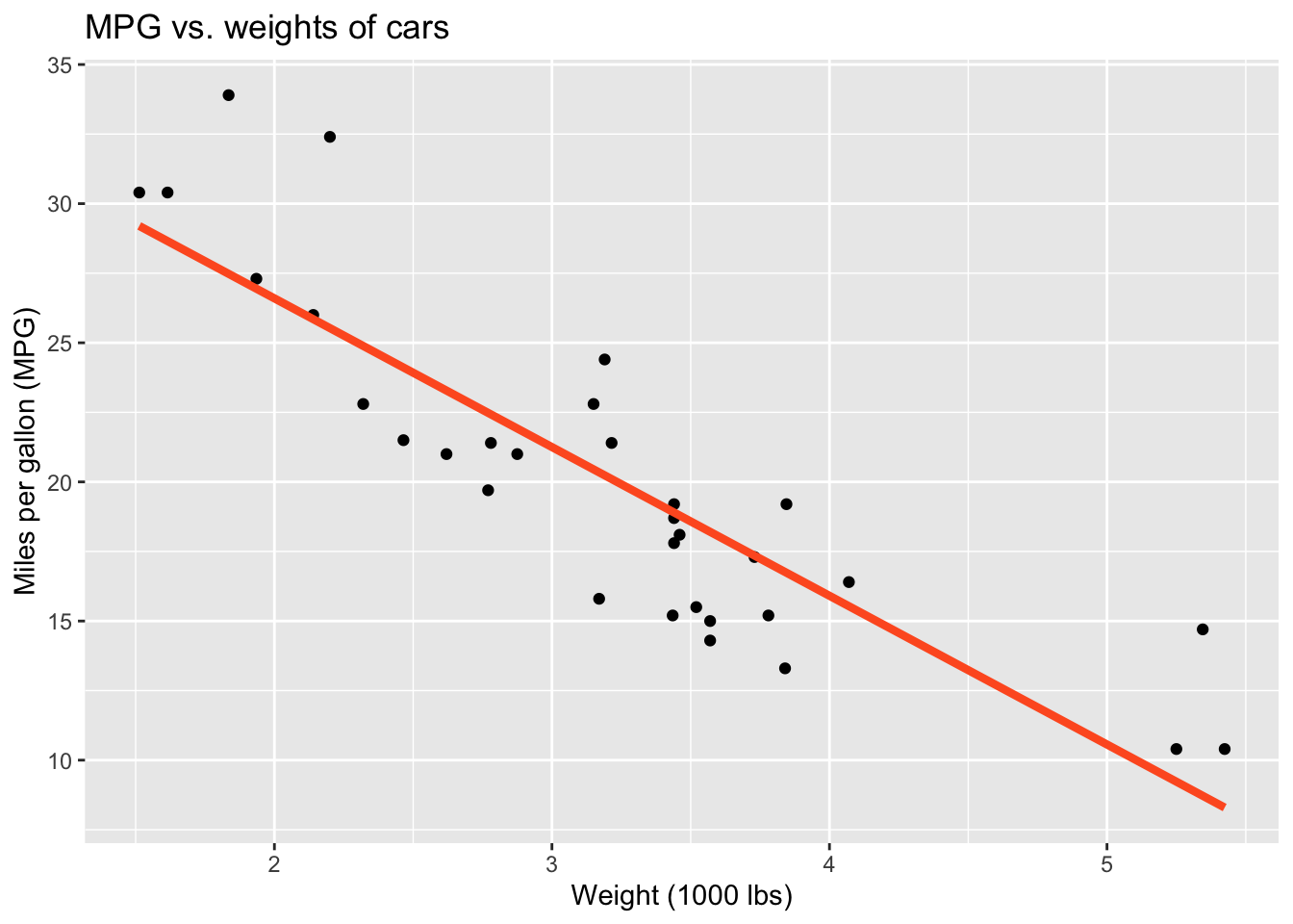
What is a line?
But on a plot…

But in math terms…
\[ \begin{aligned} y &= mx + b \\ \text{Output}&=\text{Slope}\times \text{Input} + \text{Intercept} \end{aligned} \]
Predictor (explanatory variable)
Outcome (response variable)
| mpg | wt |
|---|---|
| 21 | 2.62 |
| 21 | 2.875 |
| 22.8 | 2.32 |
| 21.4 | 3.215 |
| 18.7 | 3.44 |
| 18.1 | 3.46 |
| ... | ... |
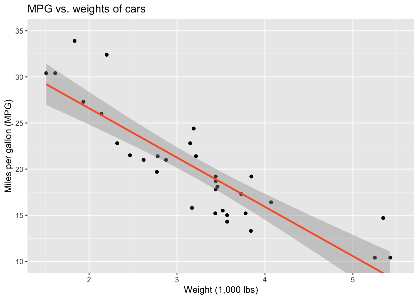
Regression line
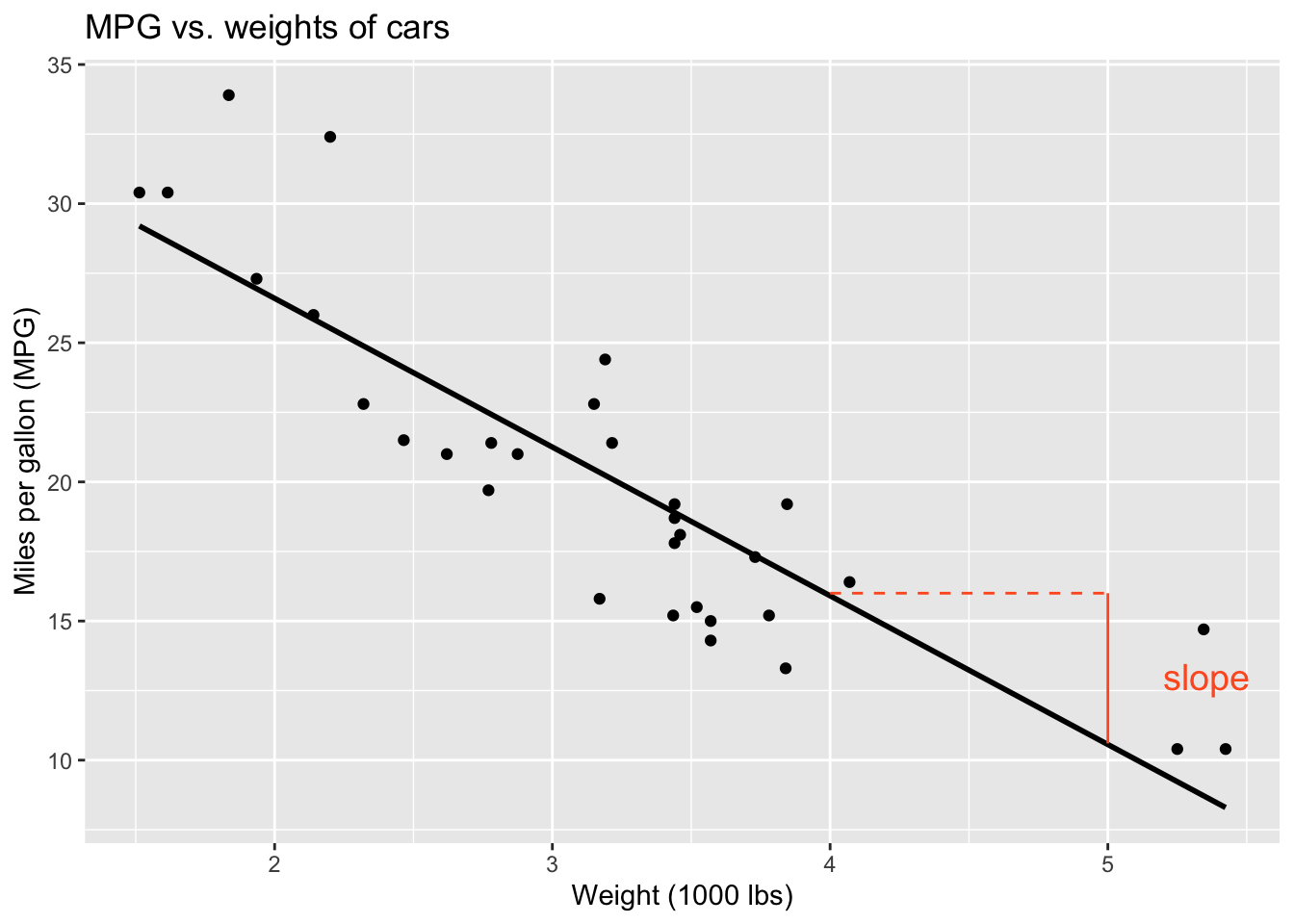
Regression line: slope
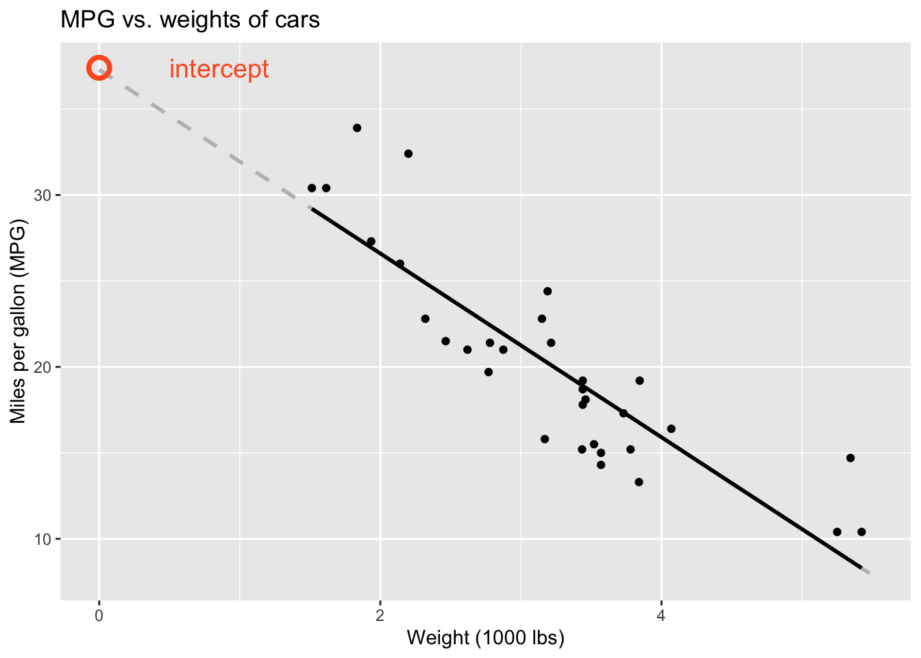
Regression line: intercept
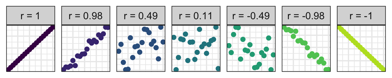
Correlation
Correlation
- Measures the strength and direction of the linear association between two numerical variables;
- Tells you how tightly the points cluster around a straight line;
- Ranges between -1 and 1;
- Same sign as the slope.
Participate 📱💻
Which of the following is the best guess for the correlation between the two variables on the plot below?
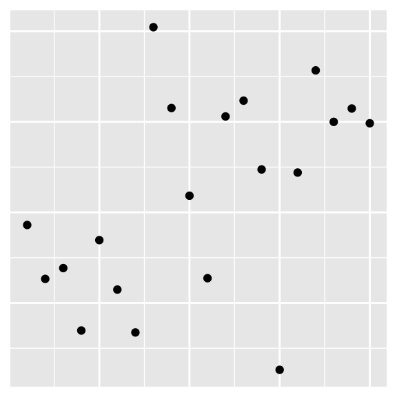
-0.95
-0.53
0.00
0.4
0.80
Scan the QR code or go HERE. Log in with your Duke NetID.
Visualizing the model
Visualizing the model
`geom_smooth()` using method = 'loess' and formula = 'y ~ x'
Visualizing the model
`geom_smooth()` using formula = 'y ~ x'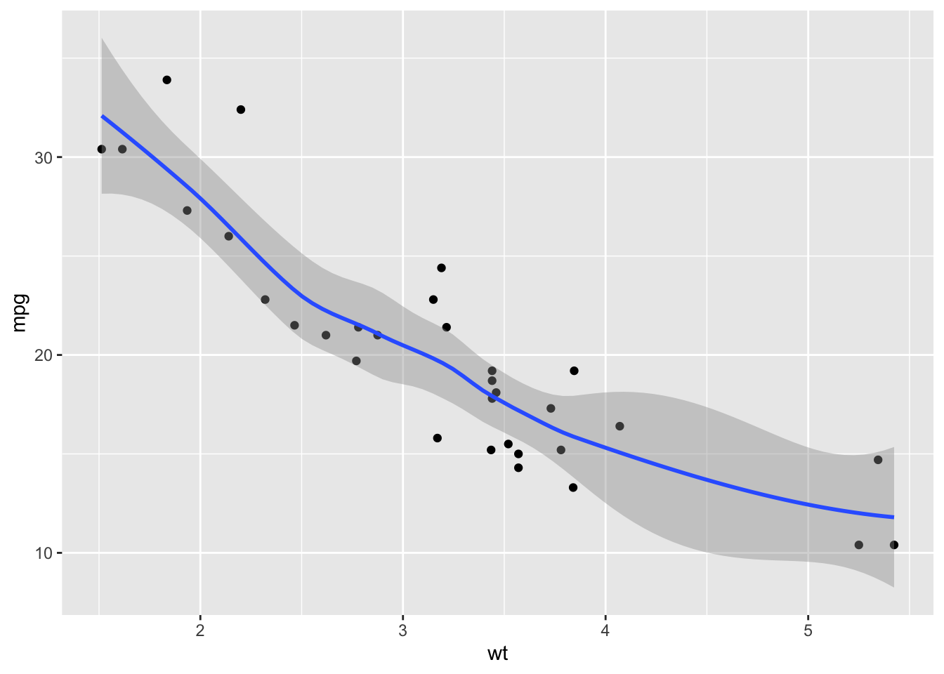
Visualizing the model
`geom_smooth()` using formula = 'y ~ x'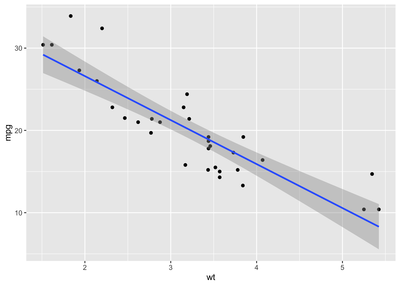
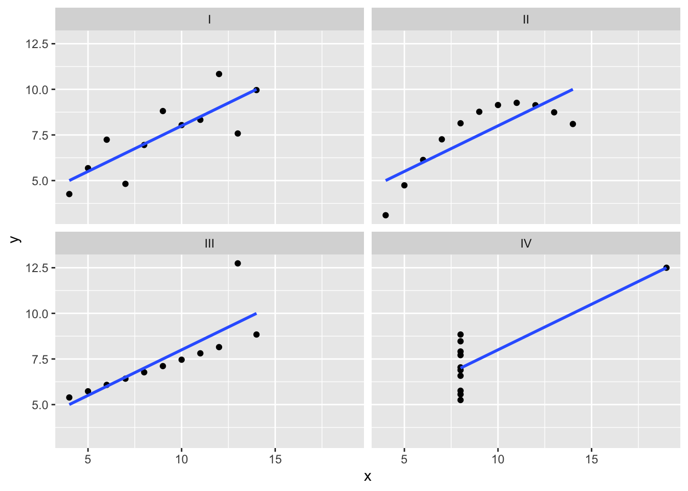
Very different
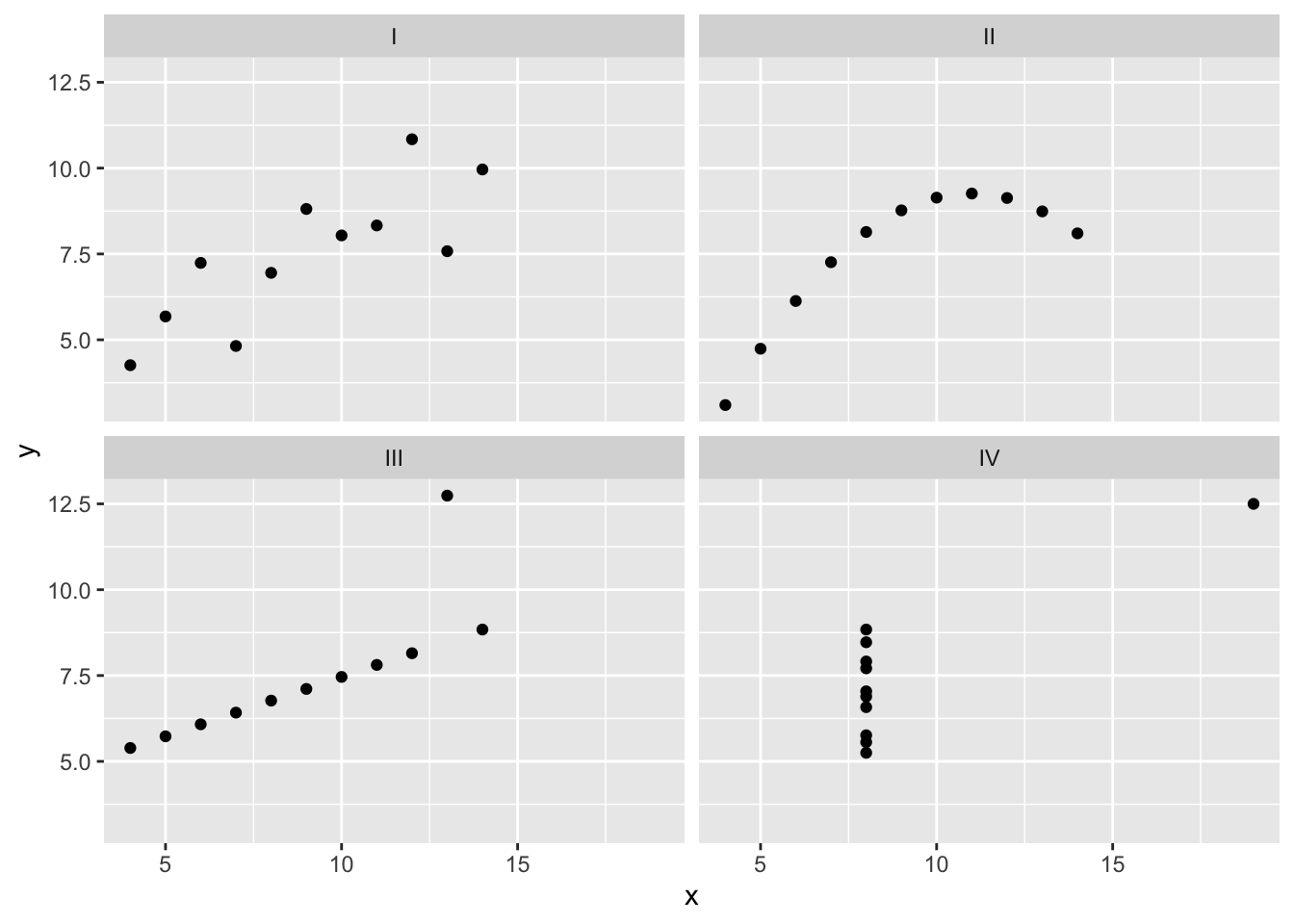
But it’s the same line…
ggplot(anscombe_tidy, aes(x, y)) +
  geom_point() +
facet_wrap(~ set) +
geom_smooth(method = "lm", se = FALSE)`geom_smooth()` using formula = 'y ~ x'