Warning: Removed 2 rows containing missing values or values outside the scale range
(`geom_point()`).Multiple Linear Regression 1
Lecture 17
2026-03-23
Do you know what Duke invests in? Neither does Nathan!

Bookbagging this Thursday!

Get great advice about course selection from the old broads in the stats mafia:
- Free boba!
- Thursday 3/26 7pm - 9pm;
- Social Sciences 136
- Instagram: @dukessmu
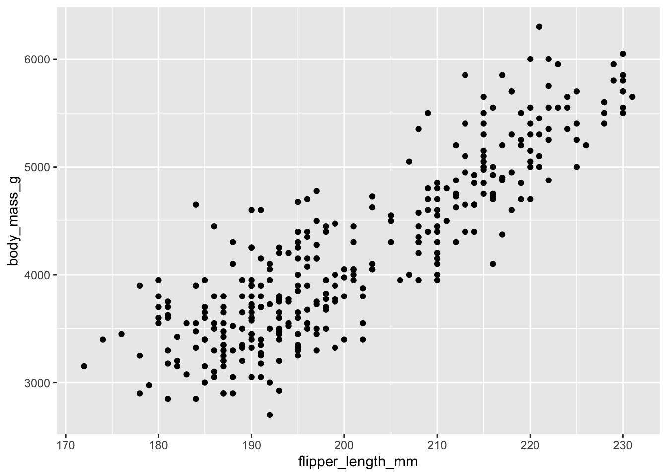
How do we concisely summarize the association between two variables?
Line of best fit!
ggplot(penguins, aes(x = flipper_length_mm, y = body_mass_g)) +
geom_point() +
geom_smooth(method = "lm")`geom_smooth()` using formula = 'y ~ x'Warning: Removed 2 rows containing non-finite outside the scale range
(`stat_smooth()`).Warning: Removed 2 rows containing missing values or values outside the scale range
(`geom_point()`).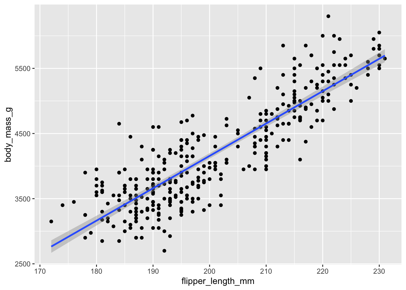
Prediction
`geom_smooth()` using formula = 'y ~ x'Warning: Removed 2 rows containing non-finite outside the scale range
(`stat_smooth()`).Warning: Removed 2 rows containing missing values or values outside the scale range
(`geom_point()`).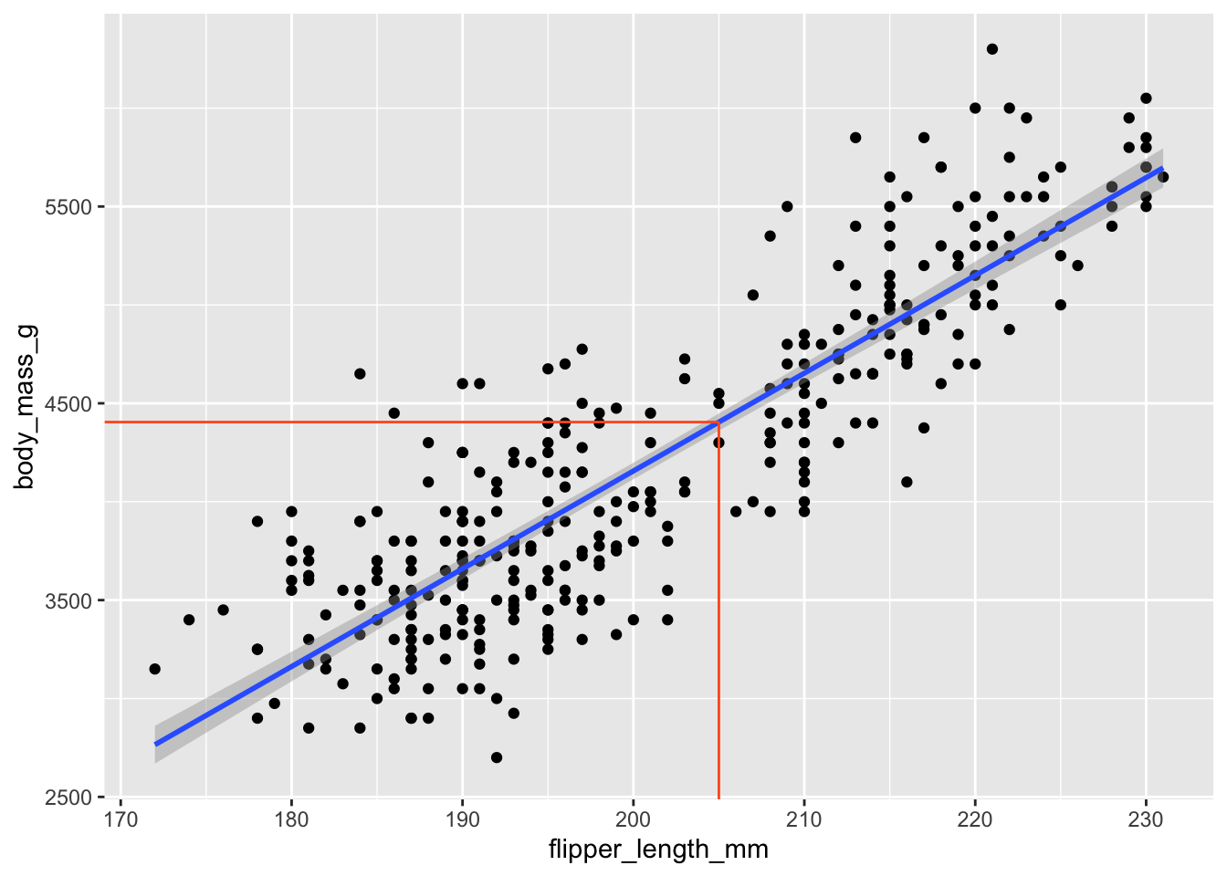
Scatterplot: possible, but not so good
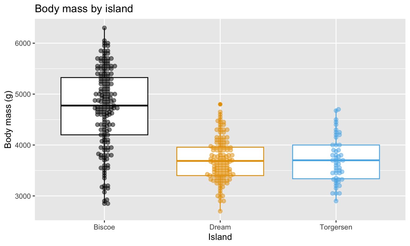
Visualize the relationship between body weight and island of penguins. Also calculate the average body weight per island.
Warning: Removed 2 rows containing missing values or values outside the scale range
(`geom_point()`).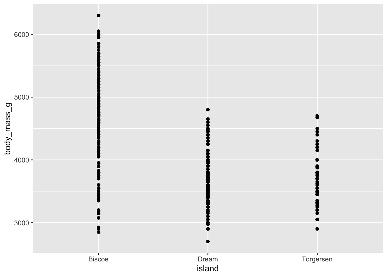
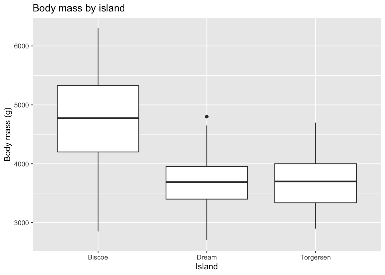
Boxplot
Visualize the relationship between body weight and island of penguins. Also calculate the average body weight per island.
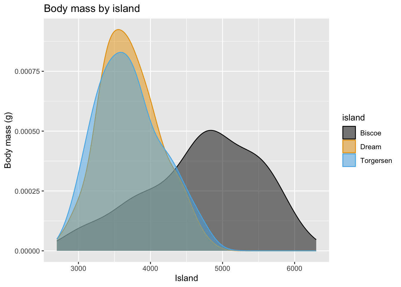
Density plot
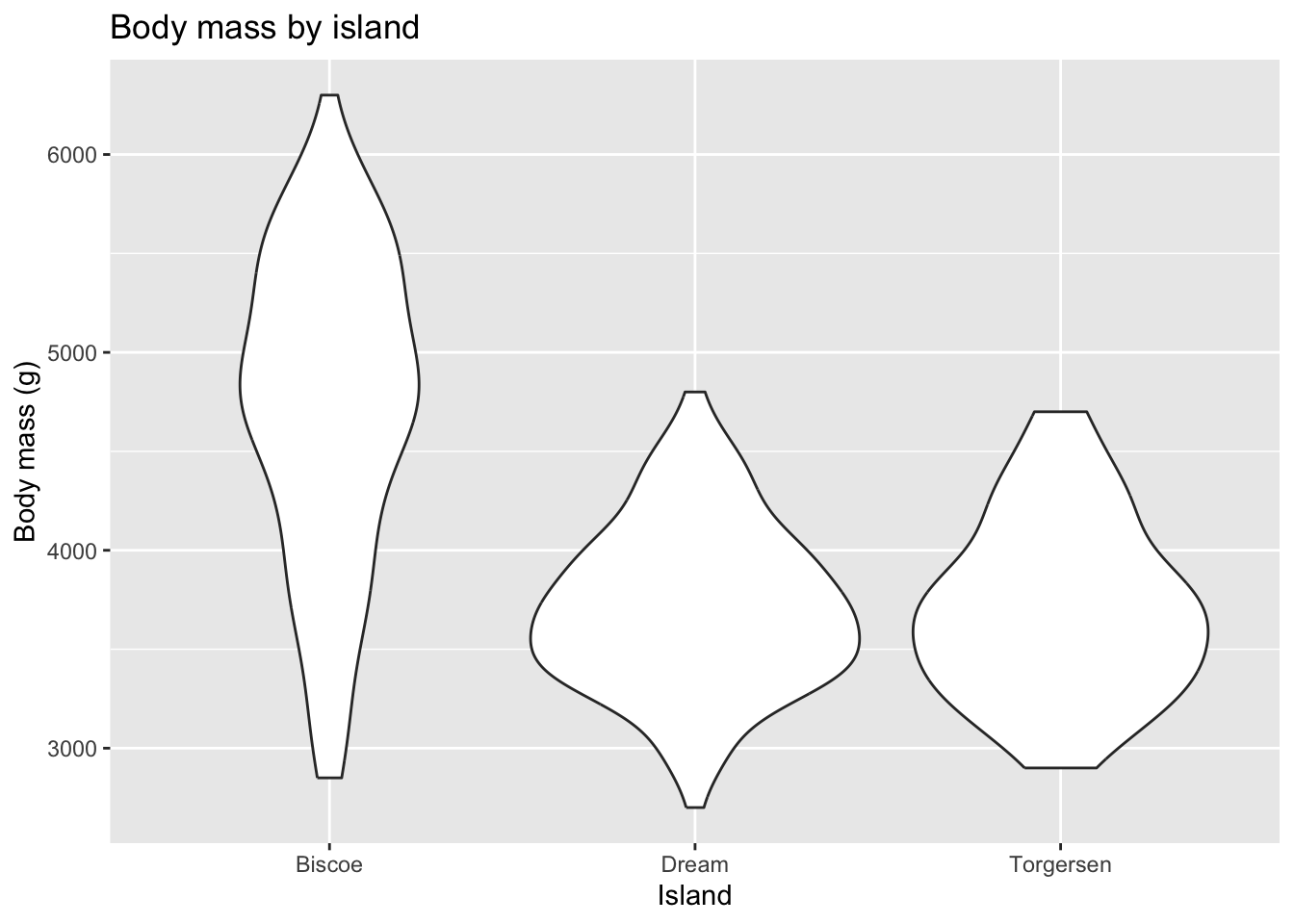
Violin plot
Multiple geoms
Three variables on one 2D plot
Warning: Removed 2 rows containing missing values or values outside the scale range
(`geom_point()`).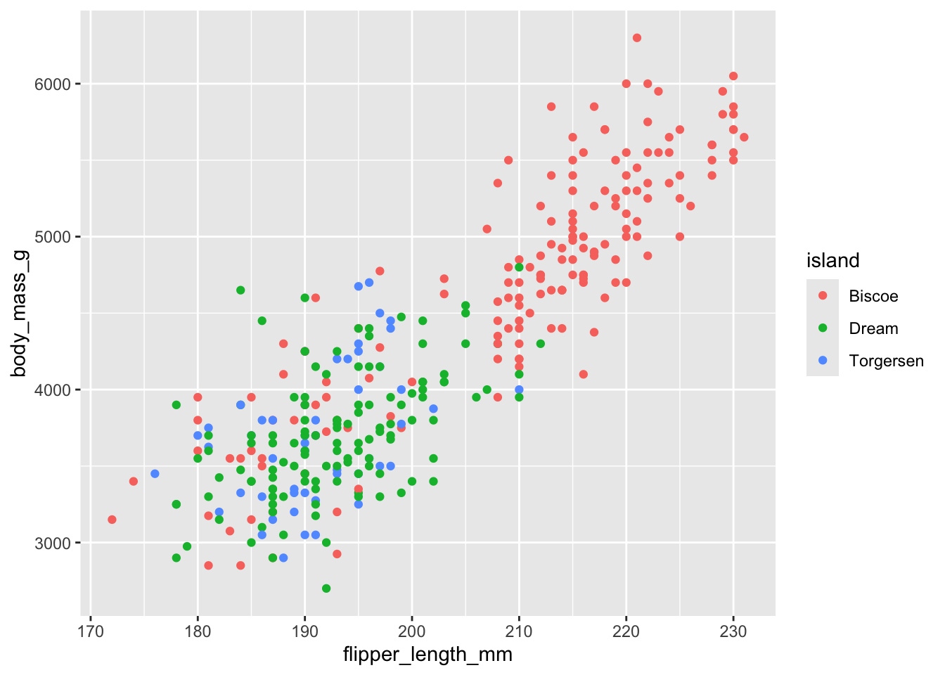
How do we predict using more than one predictor?
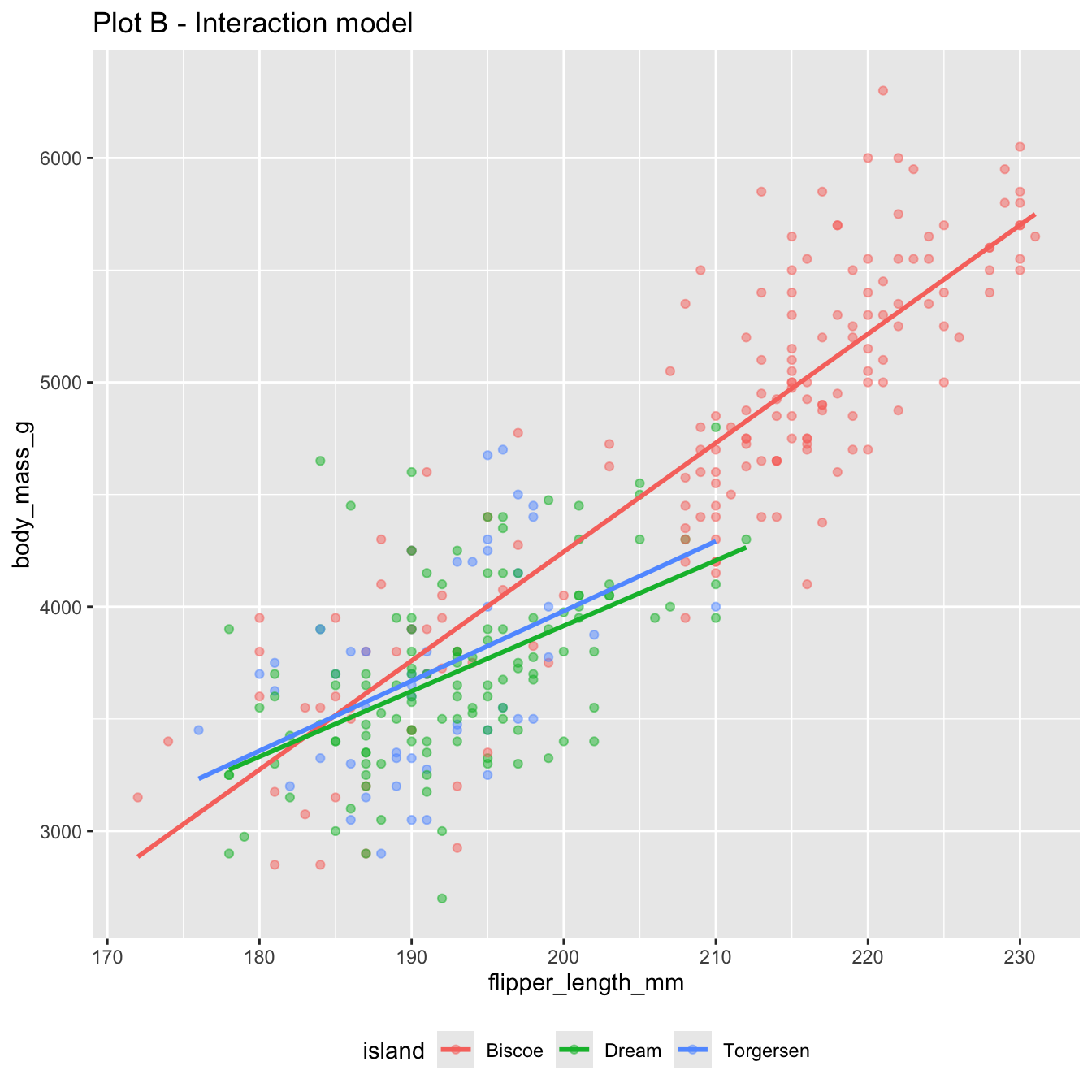
Both of these models use flipper_length_mm and island to predict body_mass_g:
`geom_smooth()` using formula = 'y ~ x'Warning: Removed 2 rows containing non-finite outside the scale range
(`stat_smooth()`).Warning: Removed 2 rows containing missing values or values outside the scale range
(`geom_point()`).`geom_smooth()` using formula = 'y ~ x'Warning: Removed 2 rows containing non-finite outside the scale range (`stat_smooth()`).
Removed 2 rows containing missing values or values outside the scale range
(`geom_point()`).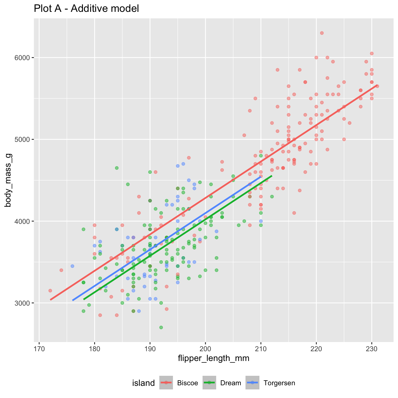
The additive model: parallel lines, one for each island
`geom_smooth()` using formula = 'y ~ x'Warning: Removed 2 rows containing non-finite outside the scale range
(`stat_smooth()`).Warning: Removed 2 rows containing missing values or values outside the scale range
(`geom_point()`).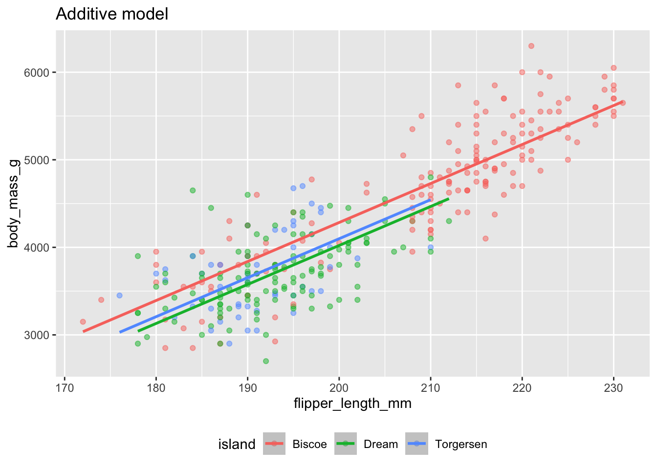
The interaction model: different lines for each island
Code
`geom_smooth()` using formula = 'y ~ x'Warning: Removed 2 rows containing non-finite outside the scale range
(`stat_smooth()`).Warning: Removed 2 rows containing missing values or values outside the scale range
(`geom_point()`).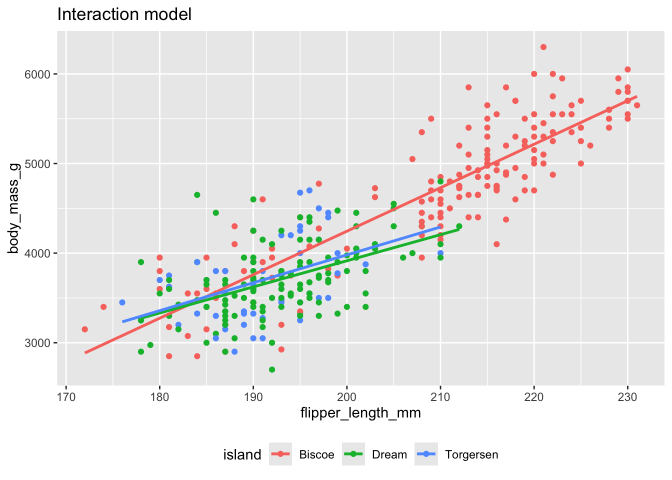
Prediction on Biscoe island
`geom_smooth()` using formula = 'y ~ x'Warning: Removed 2 rows containing non-finite outside the scale range
(`stat_smooth()`).Warning: Removed 2 rows containing missing values or values outside the scale range
(`geom_point()`).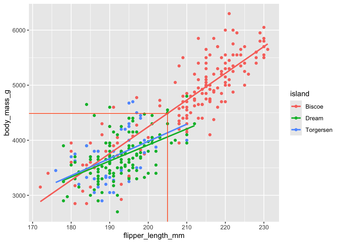
Prediction on Dream island
`geom_smooth()` using formula = 'y ~ x'Warning: Removed 2 rows containing non-finite outside the scale range
(`stat_smooth()`).Warning: Removed 2 rows containing missing values or values outside the scale range
(`geom_point()`).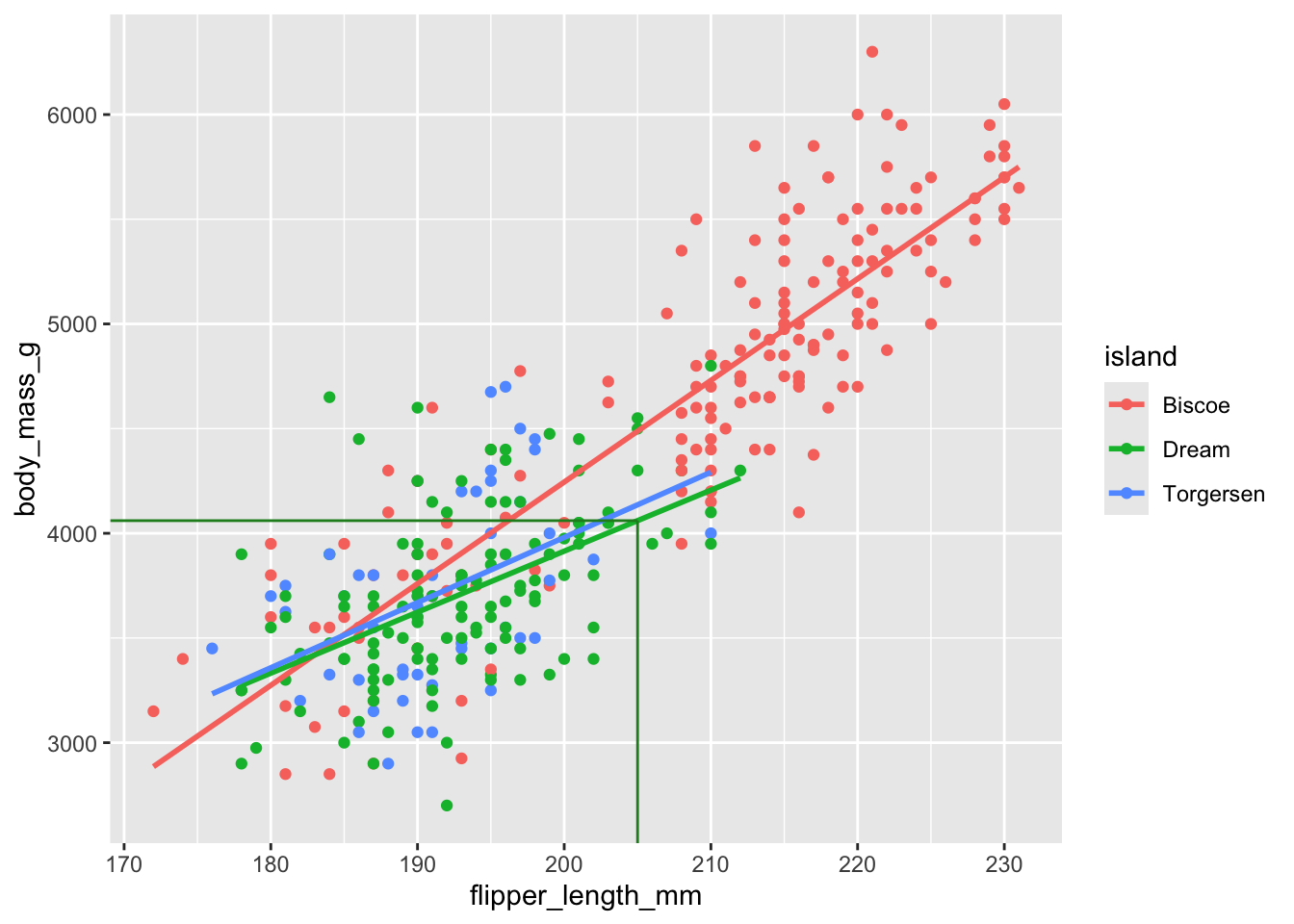
Prediction on Torgersen island
`geom_smooth()` using formula = 'y ~ x'Warning: Removed 2 rows containing non-finite outside the scale range
(`stat_smooth()`).Warning: Removed 2 rows containing missing values or values outside the scale range
(`geom_point()`).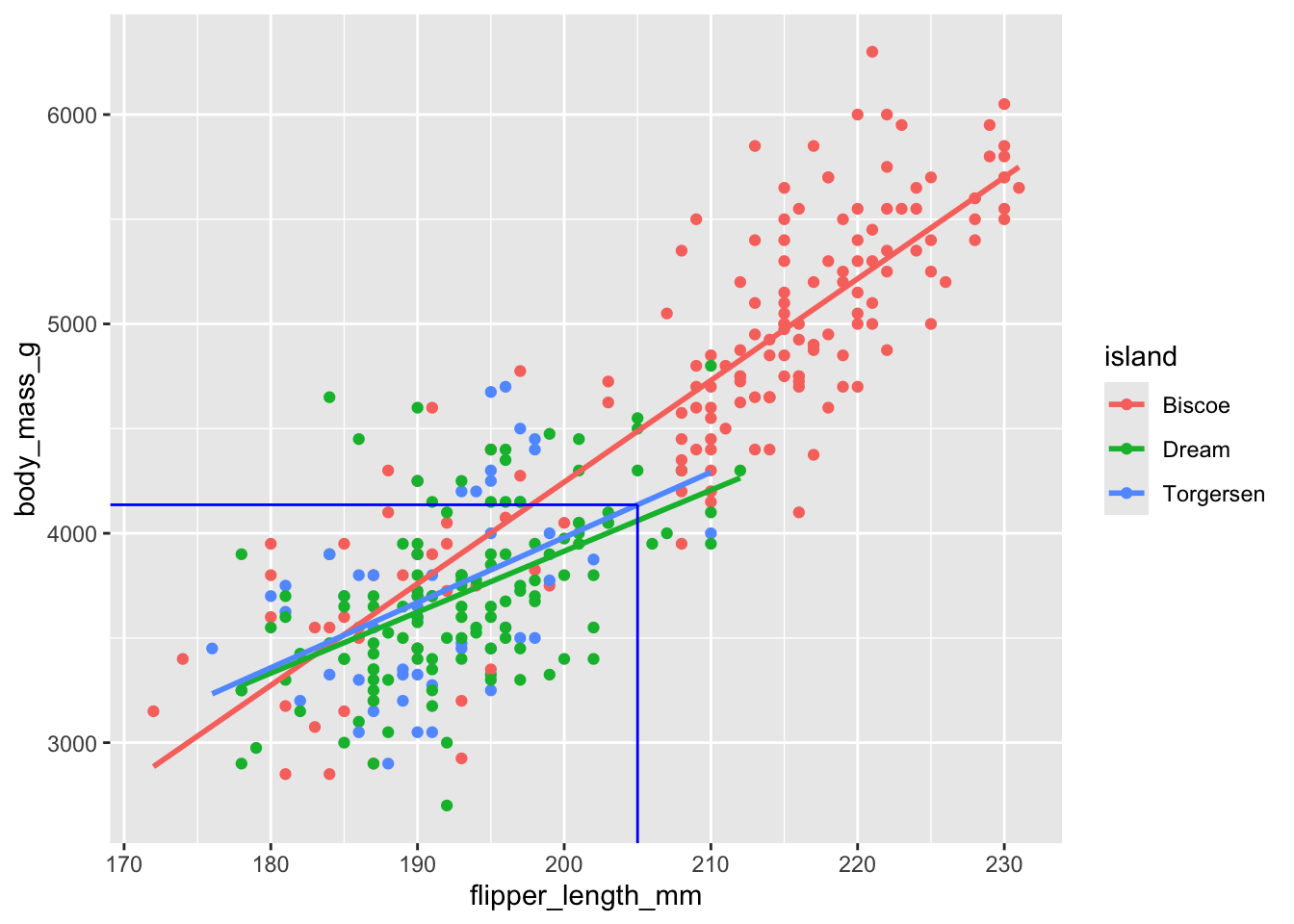
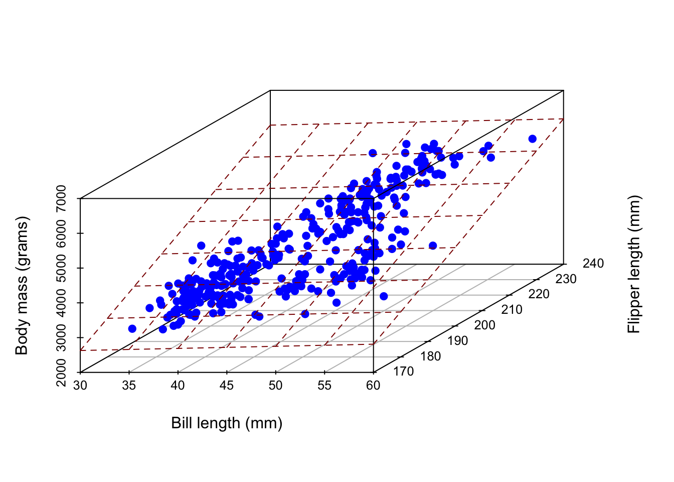
Picture? It’s not pretty…
2 predictors + 1 response = 3 dimensions. Ick!
Warning: Unknown or uninitialised column: `color`.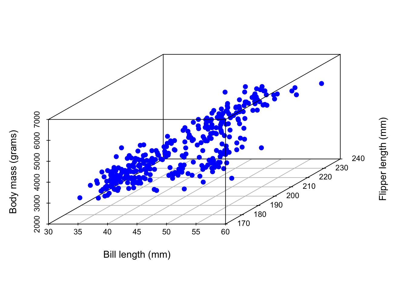
Picture? It’s not pretty…
Instead of a line of best fit, it’s a plane of best fit. Double ick!
Warning: Unknown or uninitialised column: `color`.