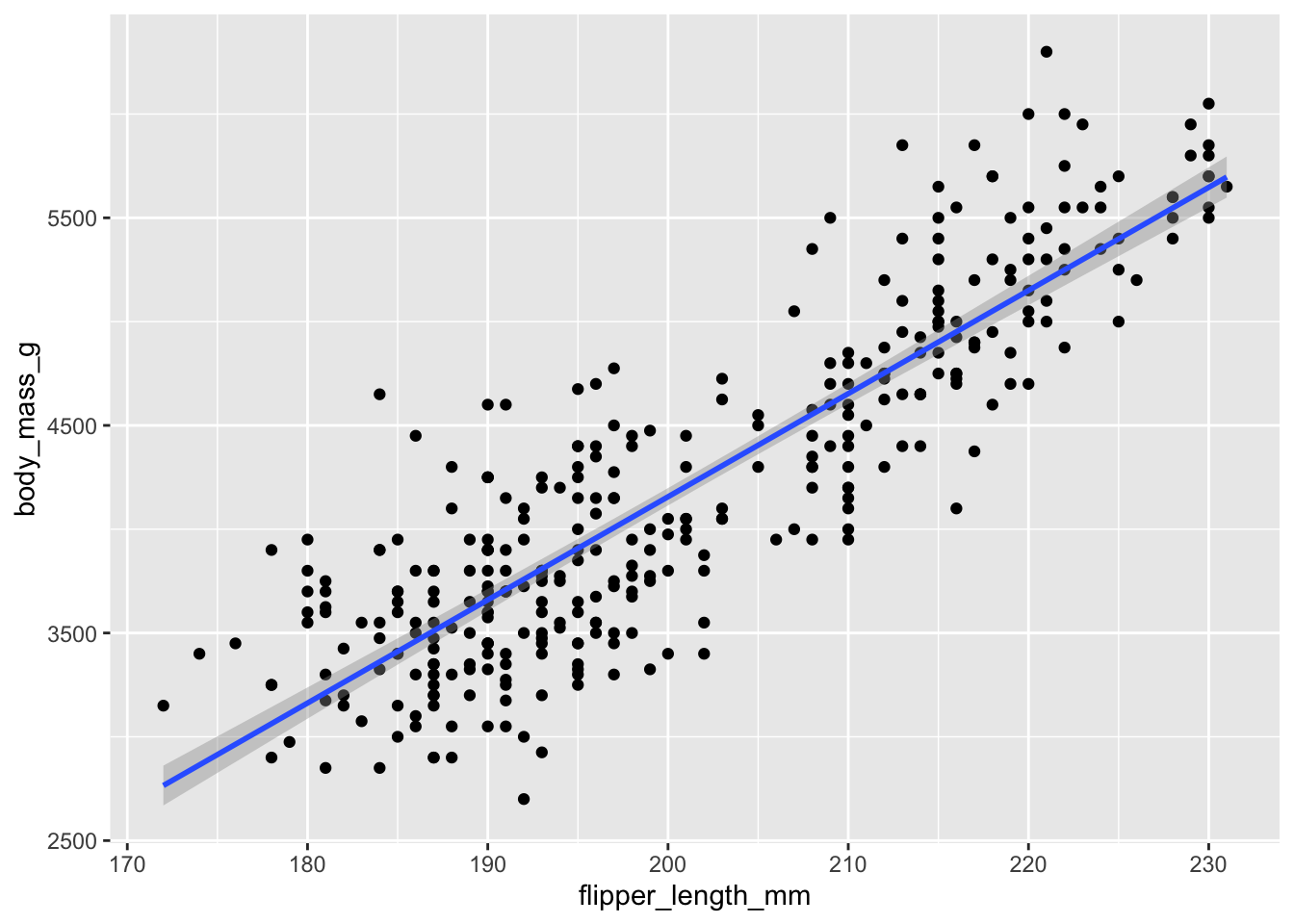
`geom_smooth()` using formula = 'y ~ x'Warning: Removed 2 rows containing non-finite outside the scale range
(`stat_smooth()`).Warning: Removed 2 rows containing missing values or values outside the scale range
(`geom_point()`).Lecture 18
2026-03-25

Get great advice about course selection from the old broads in the stats mafia:
`geom_smooth()` using formula = 'y ~ x'Warning: Removed 2 rows containing non-finite outside the scale range
(`stat_smooth()`).Warning: Removed 2 rows containing missing values or values outside the scale range
(`geom_point()`).`geom_smooth()` using formula = 'y ~ x'Warning: Removed 2 rows containing non-finite outside the scale range
(`stat_smooth()`).Warning: Removed 2 rows containing missing values or values outside the scale range
(`geom_point()`).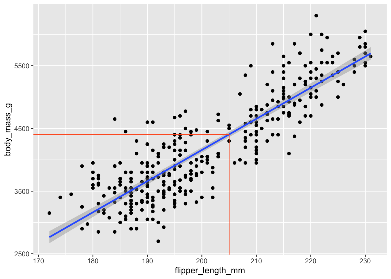
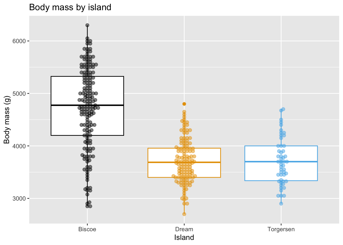
Warning: Removed 2 rows containing non-finite outside the scale range
(`stat_boxplot()`).
Warning: Removed 2 rows containing missing values or values outside the scale range
(`geom_point()`).`geom_smooth()` using formula = 'y ~ x'Warning: Removed 2 rows containing non-finite outside the scale range
(`stat_smooth()`).Warning: Removed 2 rows containing missing values or values outside the scale range
(`geom_point()`).`geom_smooth()` using formula = 'y ~ x'Warning: Removed 2 rows containing non-finite outside the scale range (`stat_smooth()`).
Removed 2 rows containing missing values or values outside the scale range
(`geom_point()`).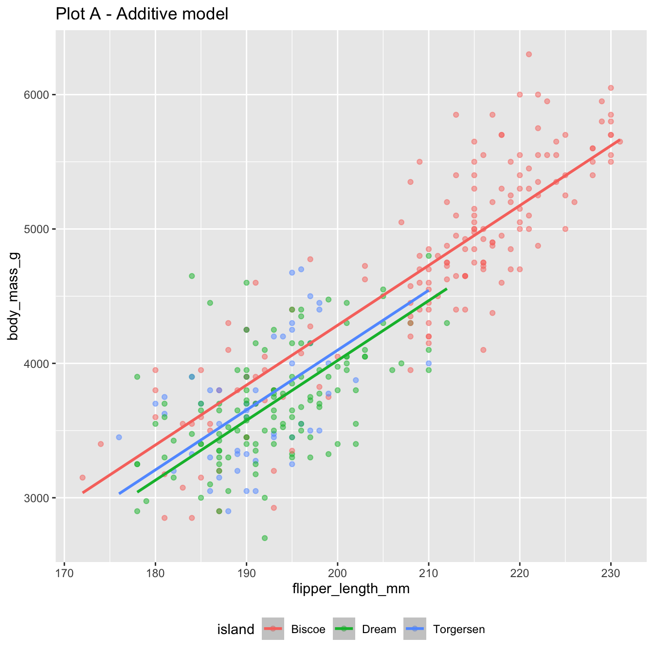
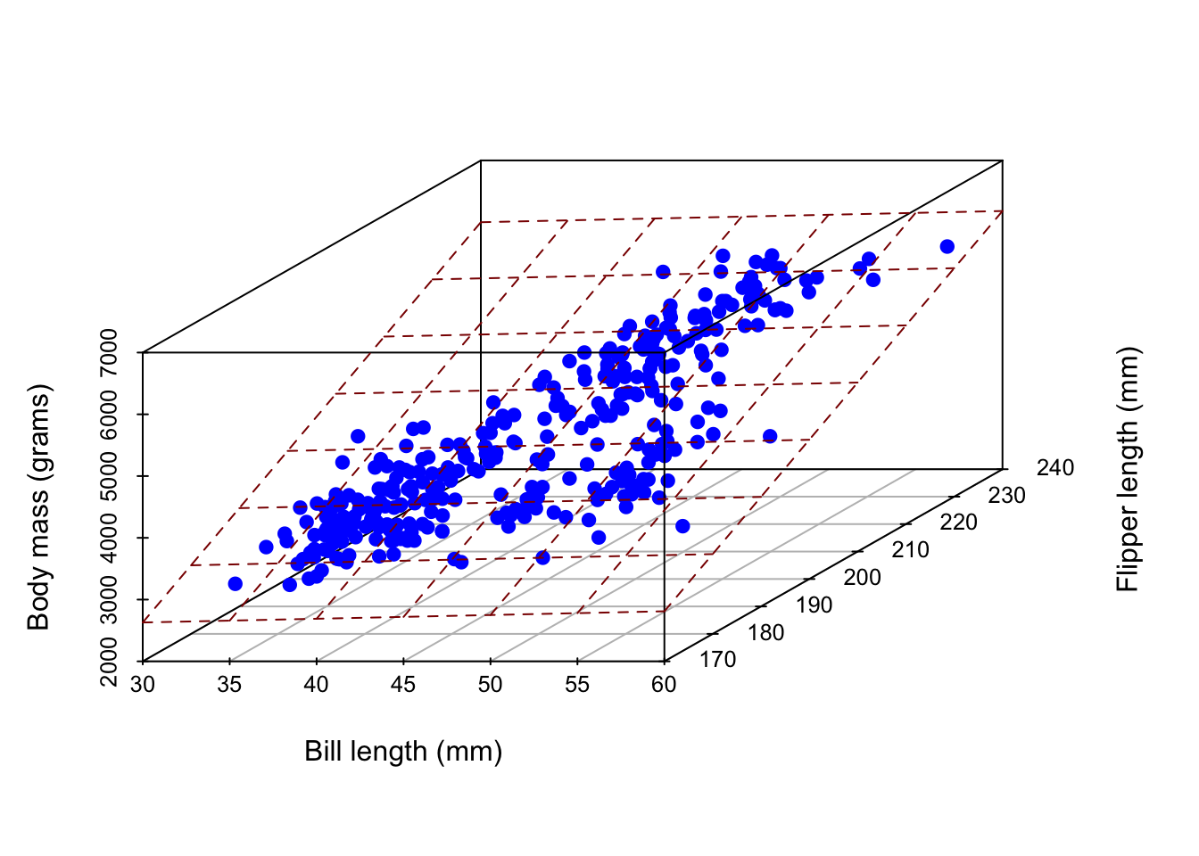
2 predictors + 1 response = 3 dimensions. Instead of a line of best fit, it’s a plane of best fit:
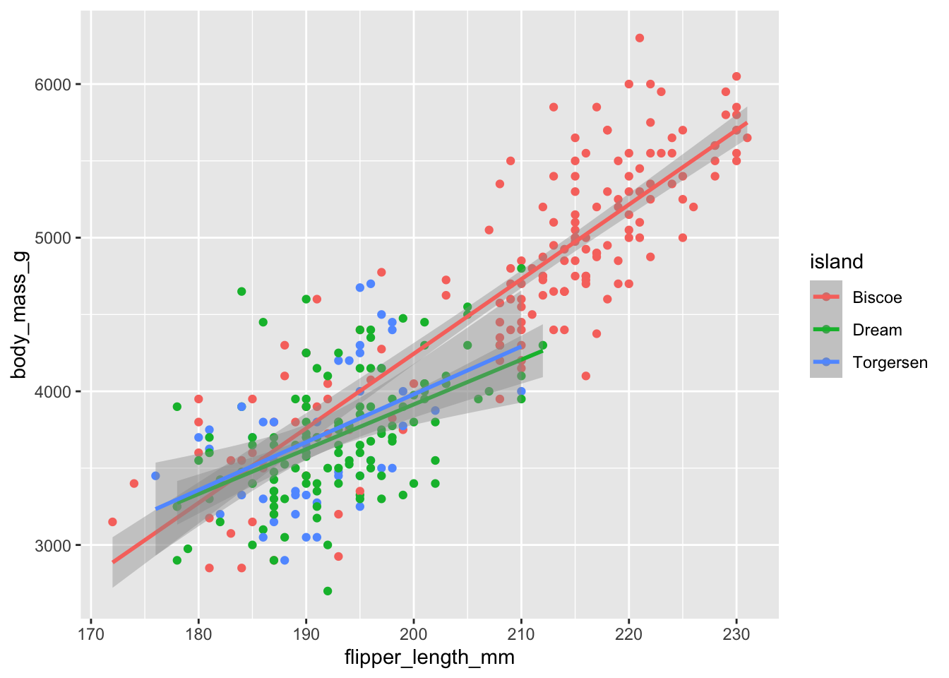
Warning: Unknown or uninitialised column: `color`.ggplot(penguins, aes(x = flipper_length_mm, y = body_mass_g, color = island)) +
geom_point() +
geom_smooth(method = "lm")`geom_smooth()` using formula = 'y ~ x'Warning: Removed 2 rows containing non-finite outside the scale range
(`stat_smooth()`).Warning: Removed 2 rows containing missing values or values outside the scale range
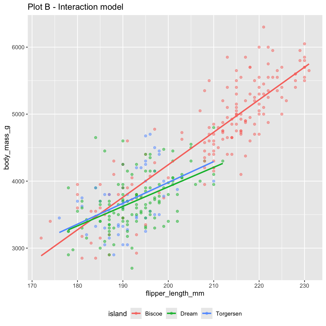
(`geom_point()`).These are separate simple regressions within each group. The slopes and the intercepts are the same as the interaction model, but the uncertainty bands are different.
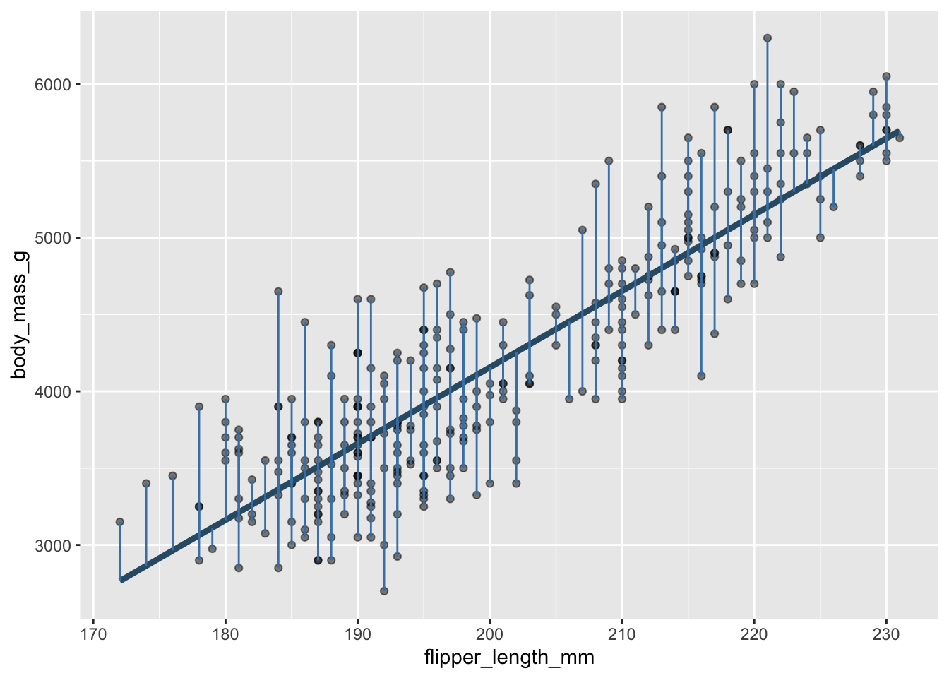
Every data point has one:
Some are big, some are small. Some are above the line (positive), and some are below the line (negative).
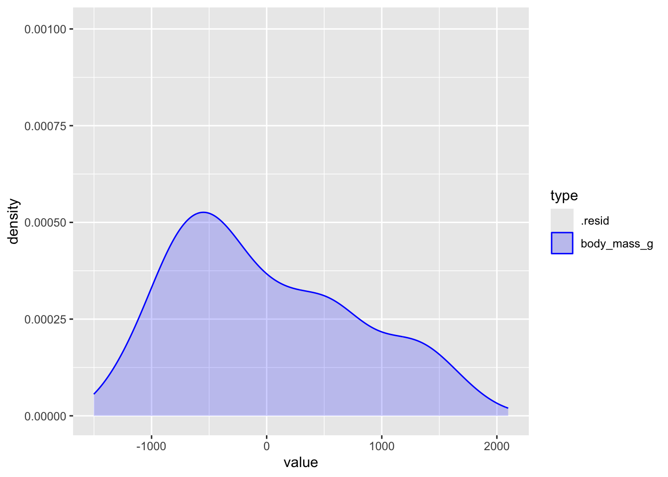
The original distribution of the response. This is the mess we’re trying to clean up with a model:
# A tibble: 1 × 3
  type        variance   std
  <chr>          <dbl> <dbl>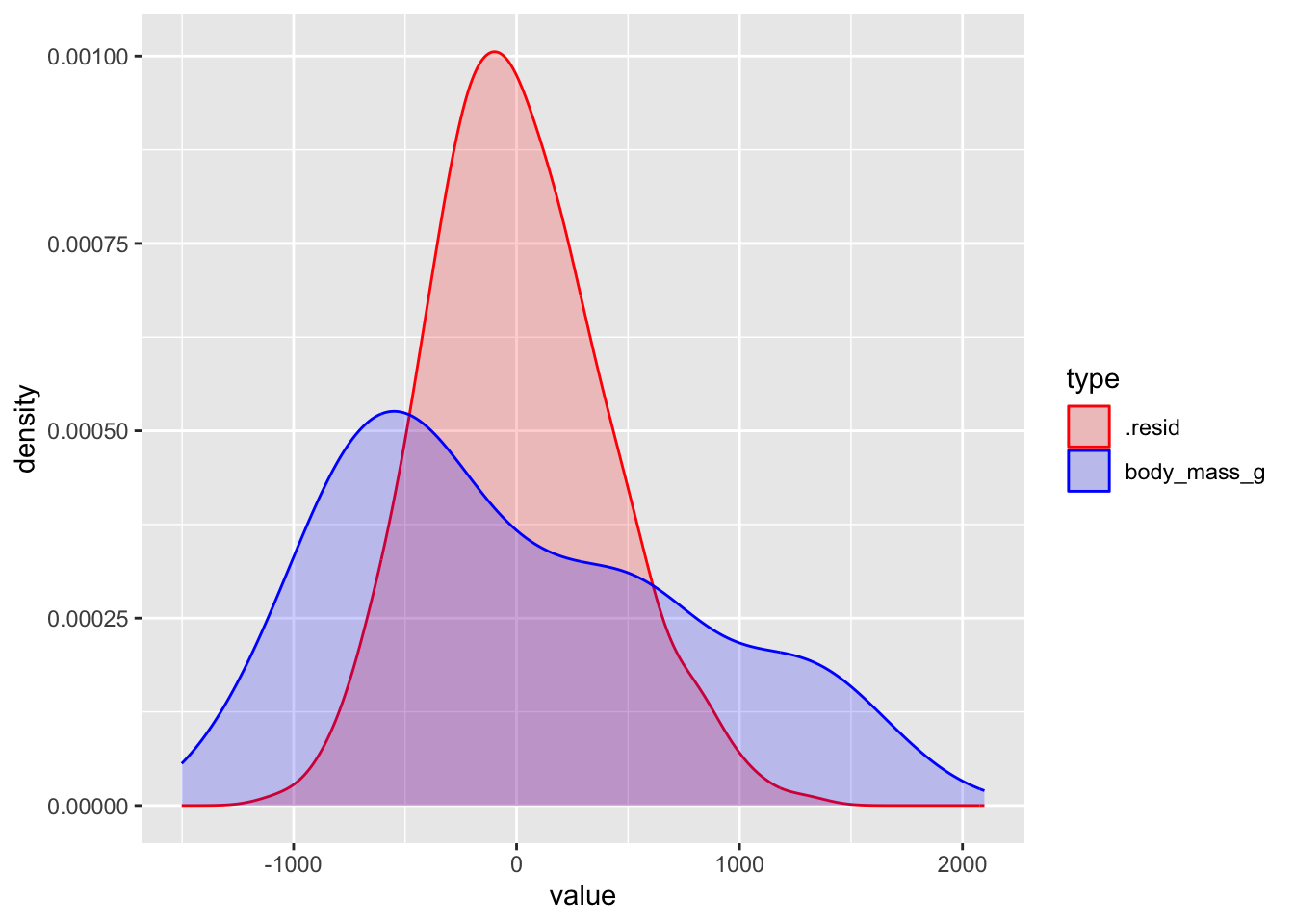
1 body_mass_g 643131. 802.The distribution of the residuals (the leftover mess) after the model tries to explain (clean up):
# A tibble: 2 × 3
type variance std
<chr> <dbl> <dbl>
1 .resid 154999. 394.
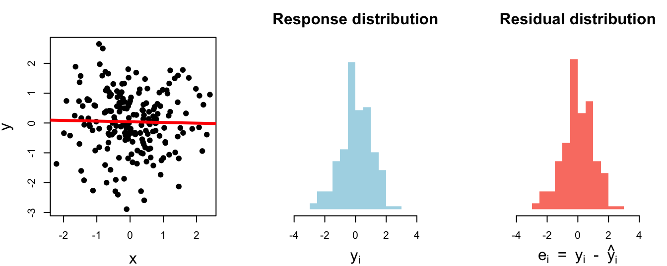
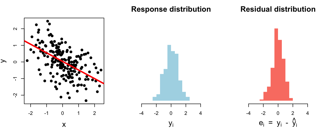
2 body_mass_g 643131. 802.Horrifically awful fit. The model didn’t explain (clean up) anything:
# A tibble: 1 × 3
  var_y var_resid r.squared
  <dbl>     <dbl>     <dbl>
1 1.02 1.02 0.000450# A tibble: 1 × 3
var_y var_resid r.squared
<dbl> <dbl> <dbl>
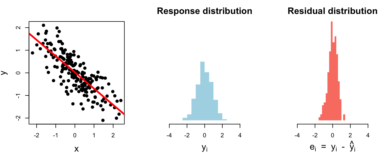
1 0.805 0.574 0.287# A tibble: 1 × 3
var_y var_resid r.squared
<dbl> <dbl> <dbl>
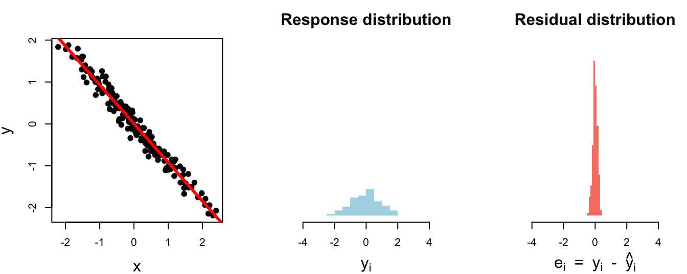
1 0.701 0.255 0.636# A tibble: 1 × 3
var_y var_resid r.squared
<dbl> <dbl> <dbl>
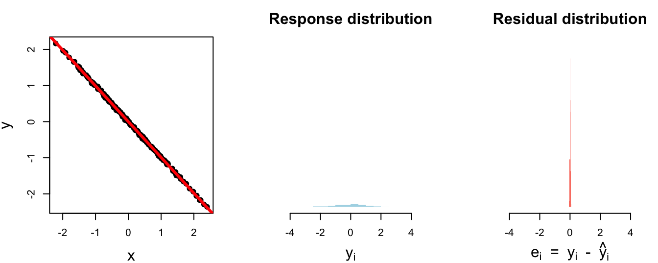
1 0.762 0.0230 0.970Perfect fit. The model explained (cleaned up) everything:
# A tibble: 1 × 3
  var_y var_resid r.squared
  <dbl>     <dbl>     <dbl>
1 0.847  0.000408     1.000