Interval estimation
Lecture 22
2026-04-13
Also

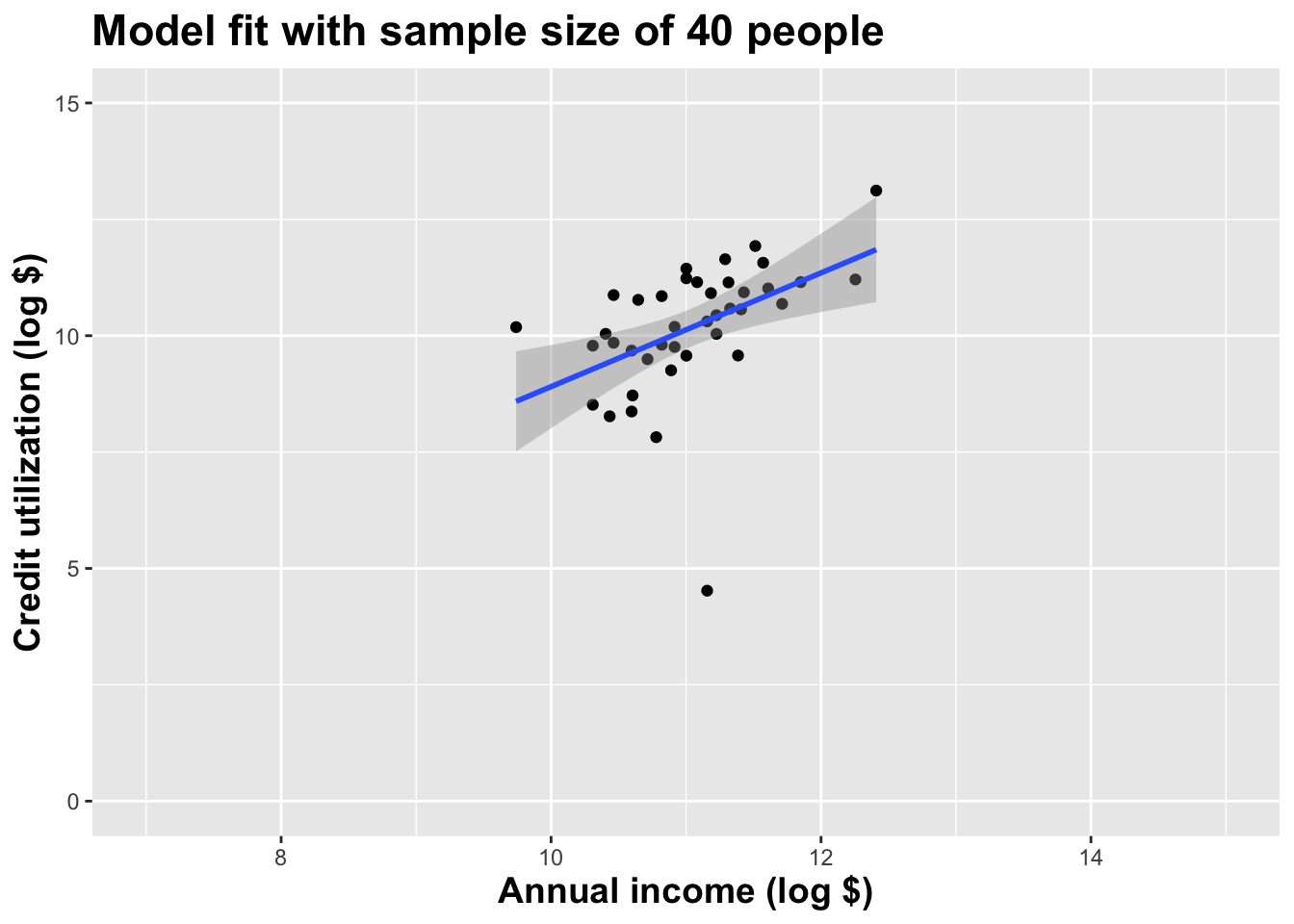
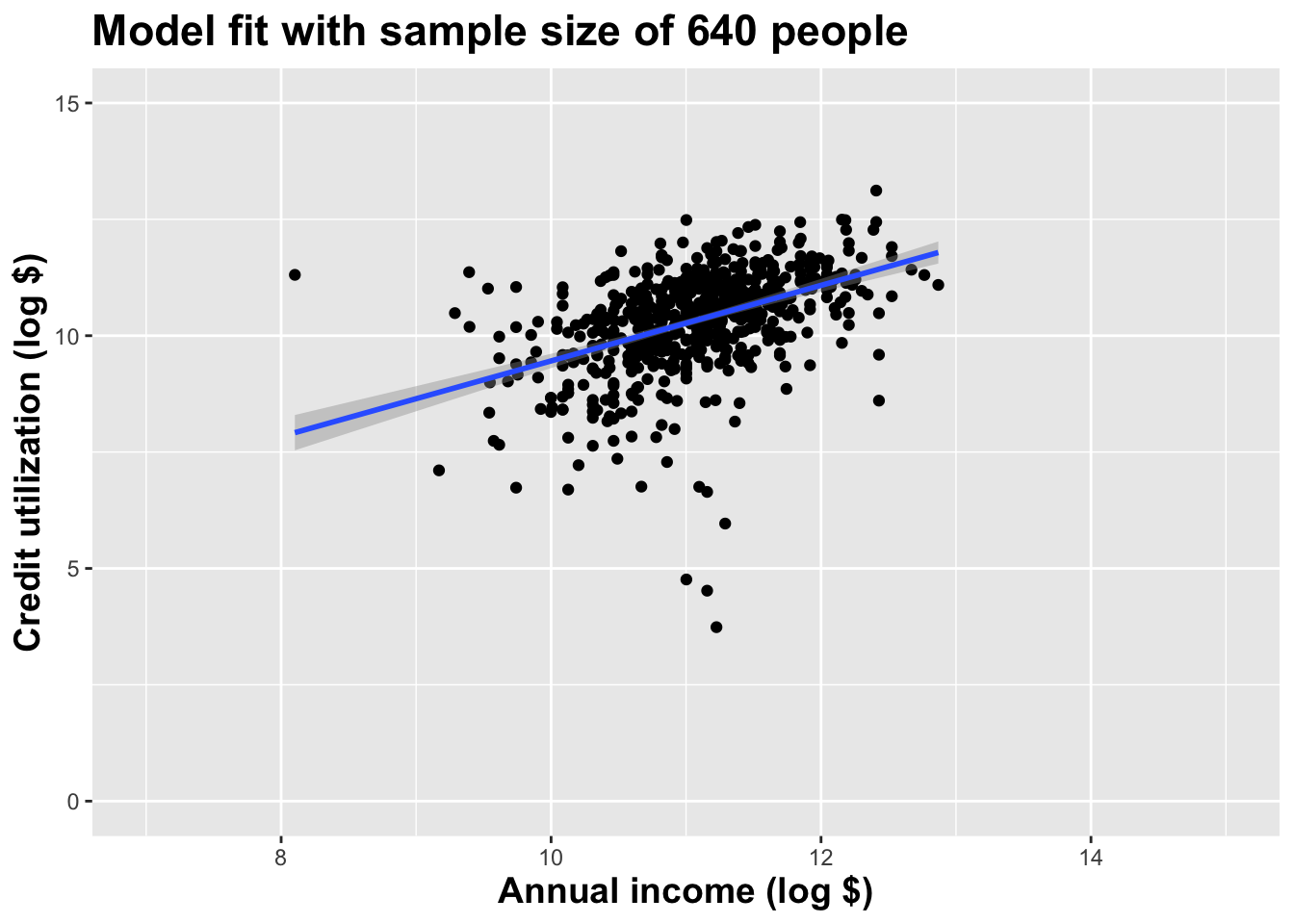
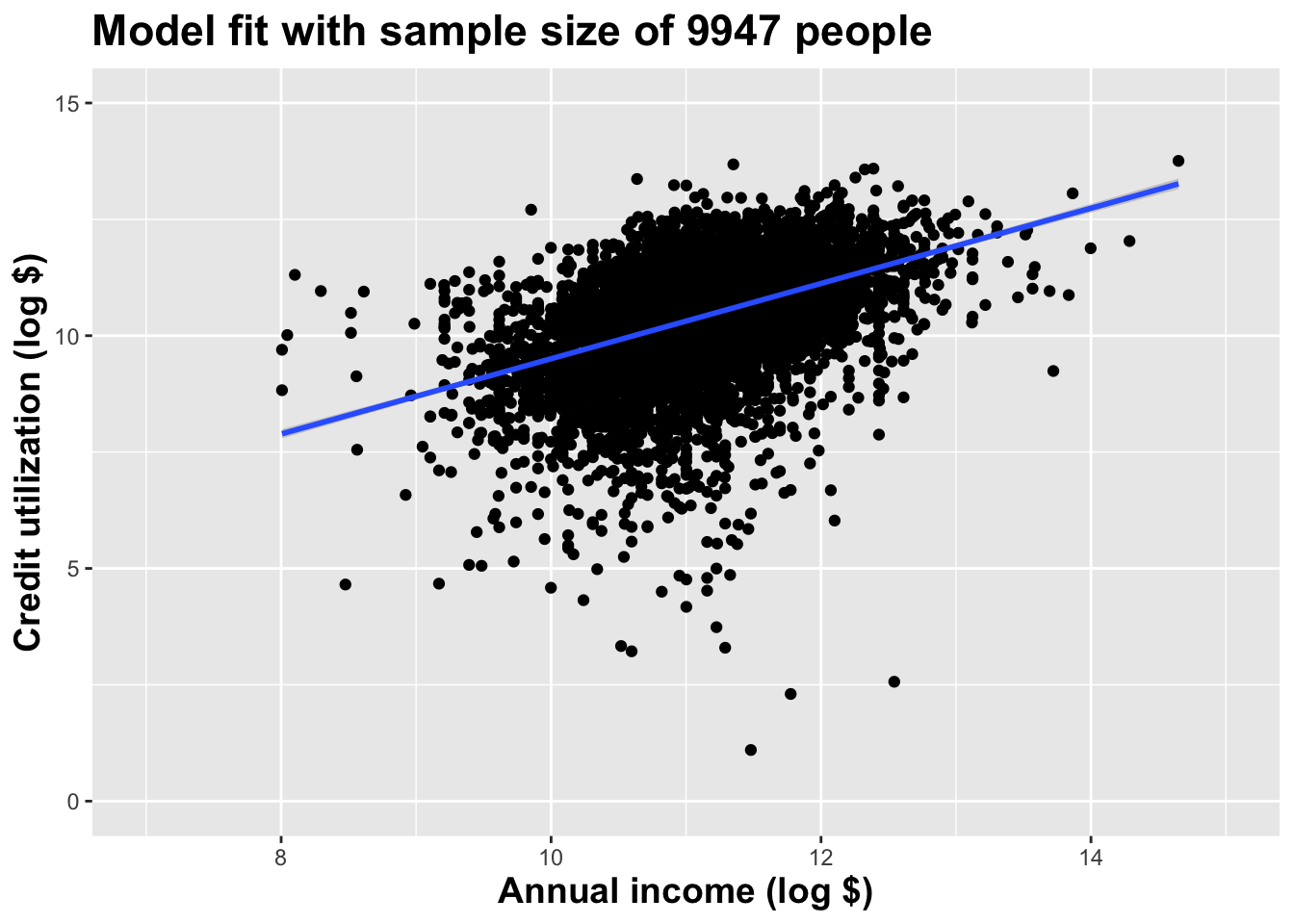
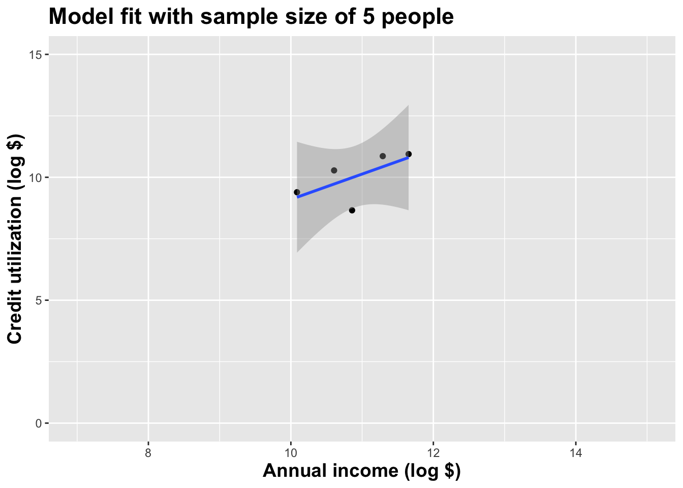
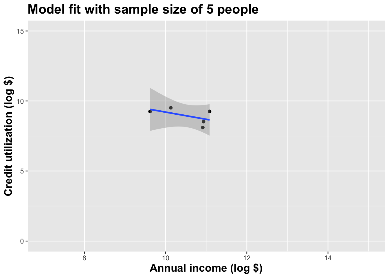
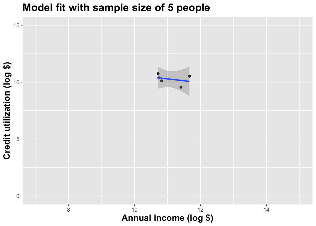
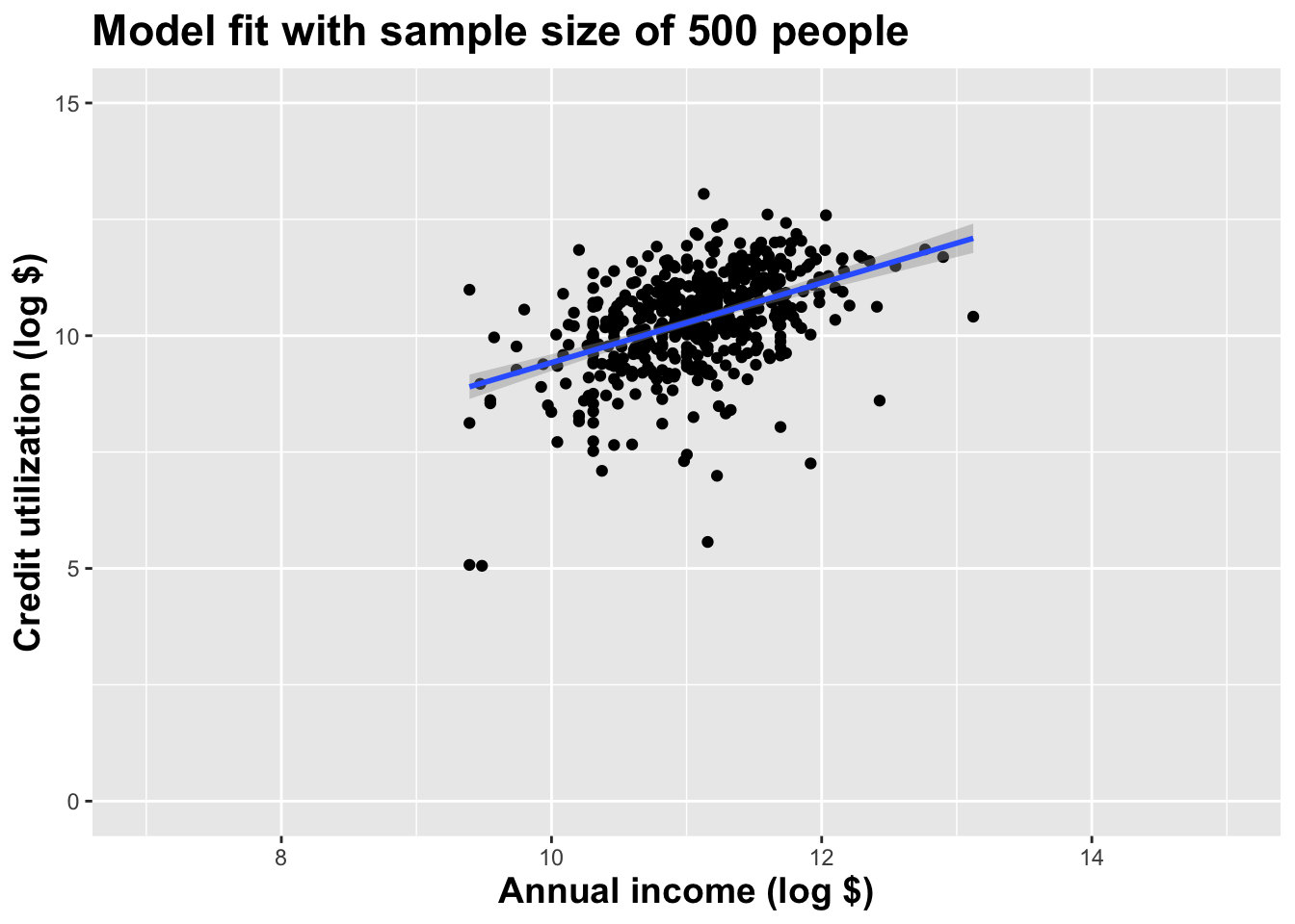
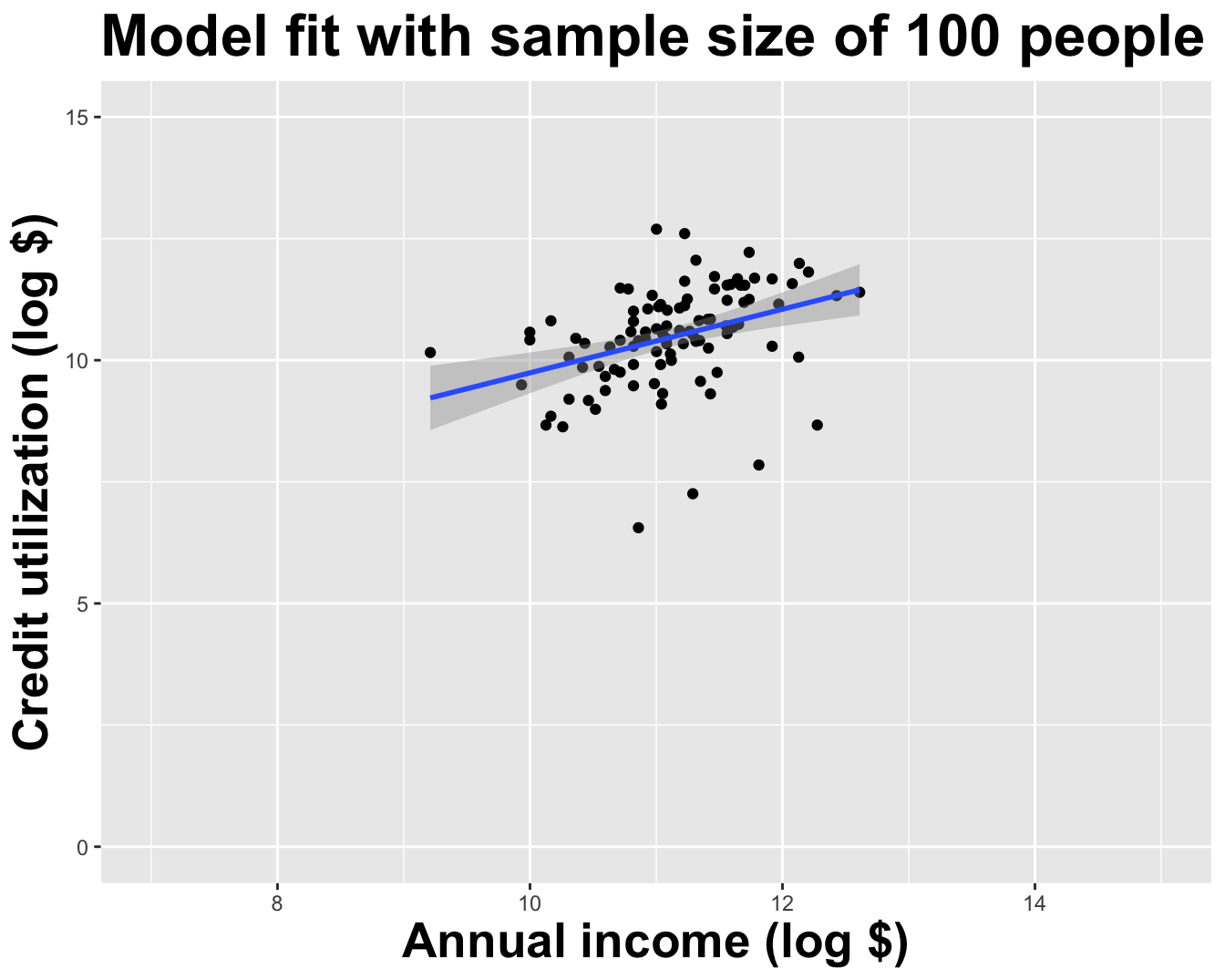
Model fit with five observations
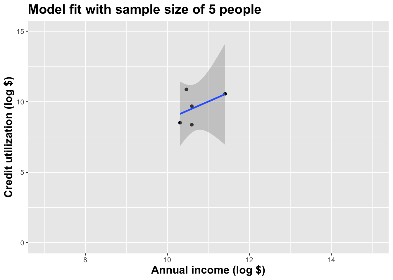
(I just took logs to make the picture prettier.)
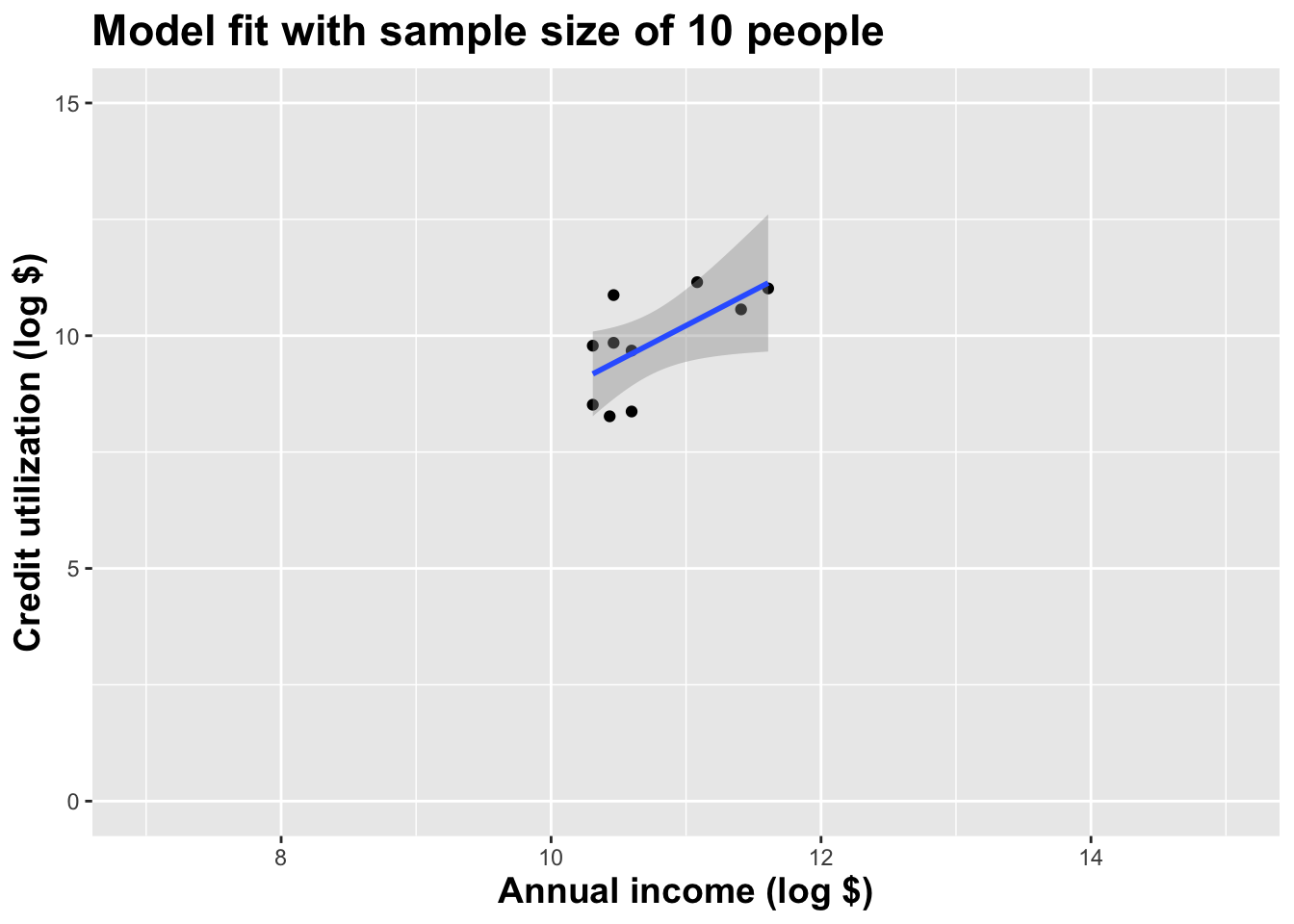
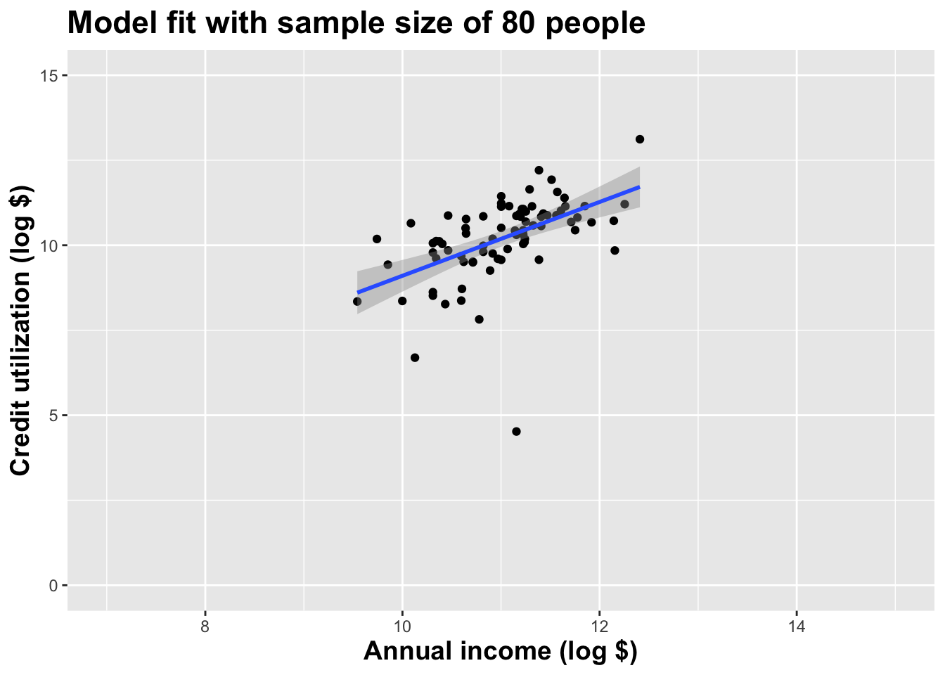
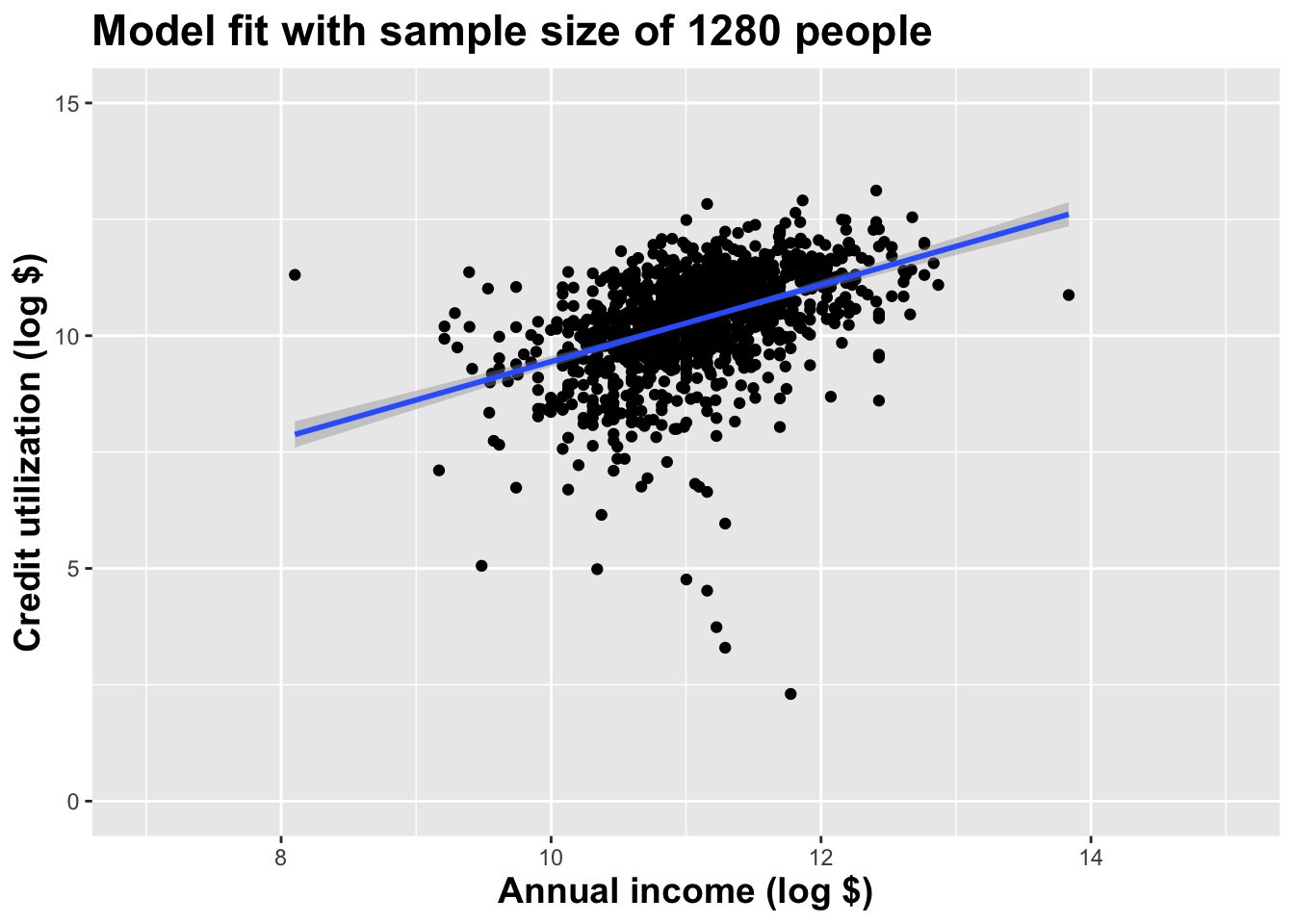
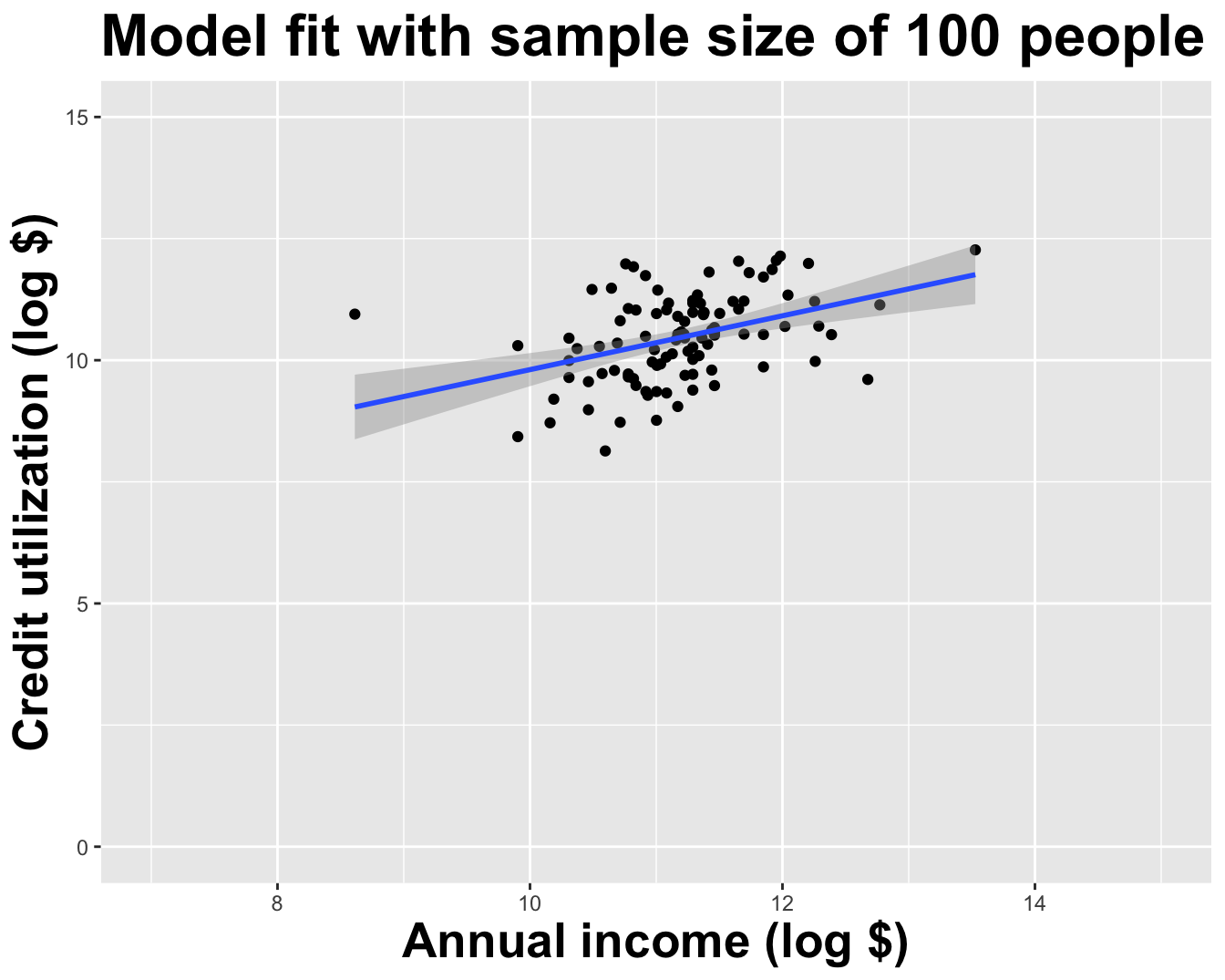
Double the sample size
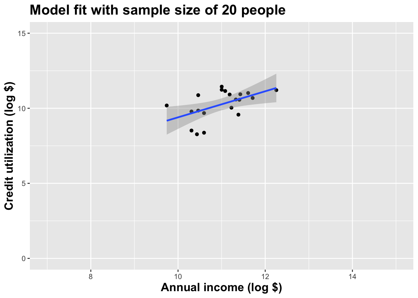
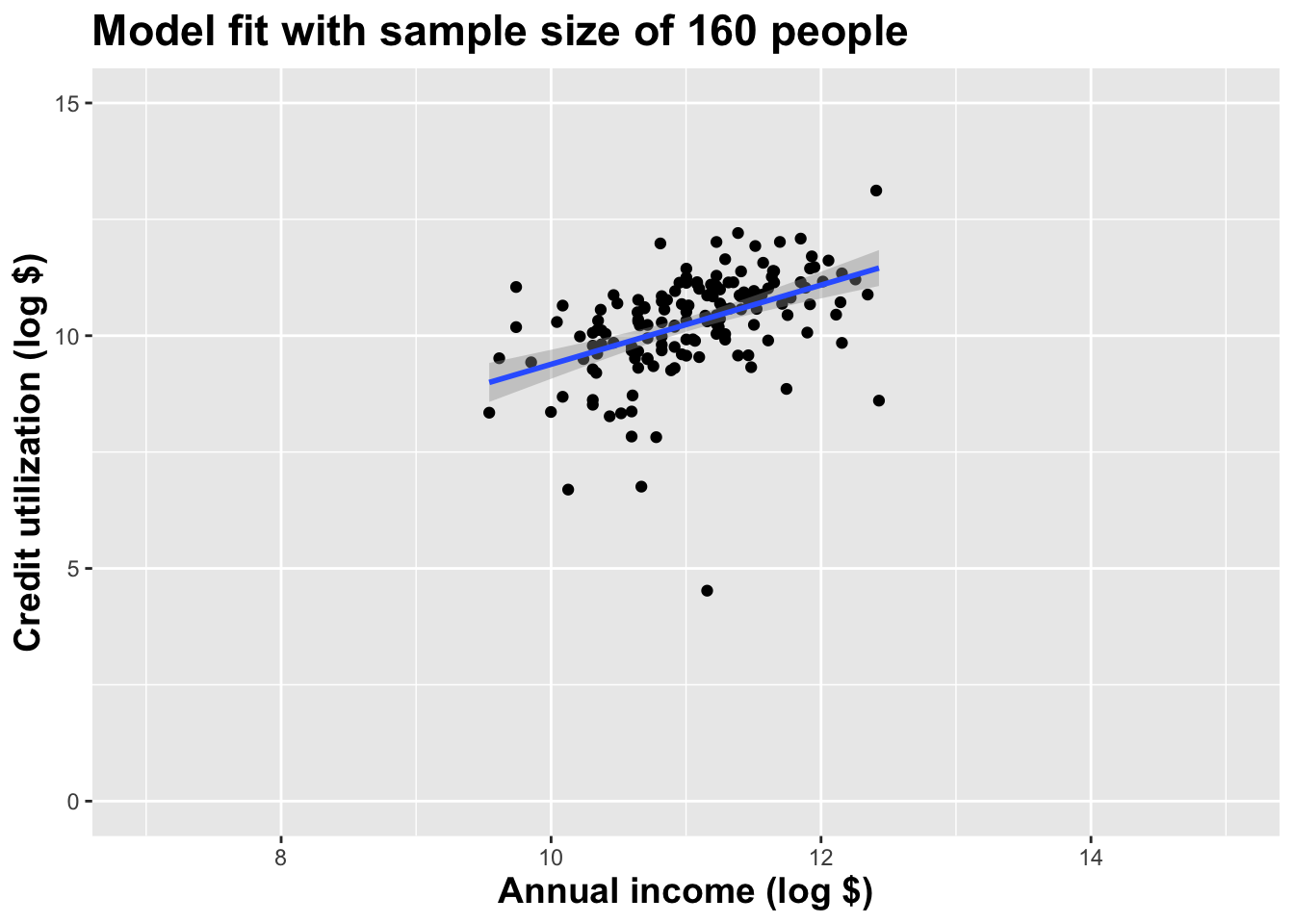
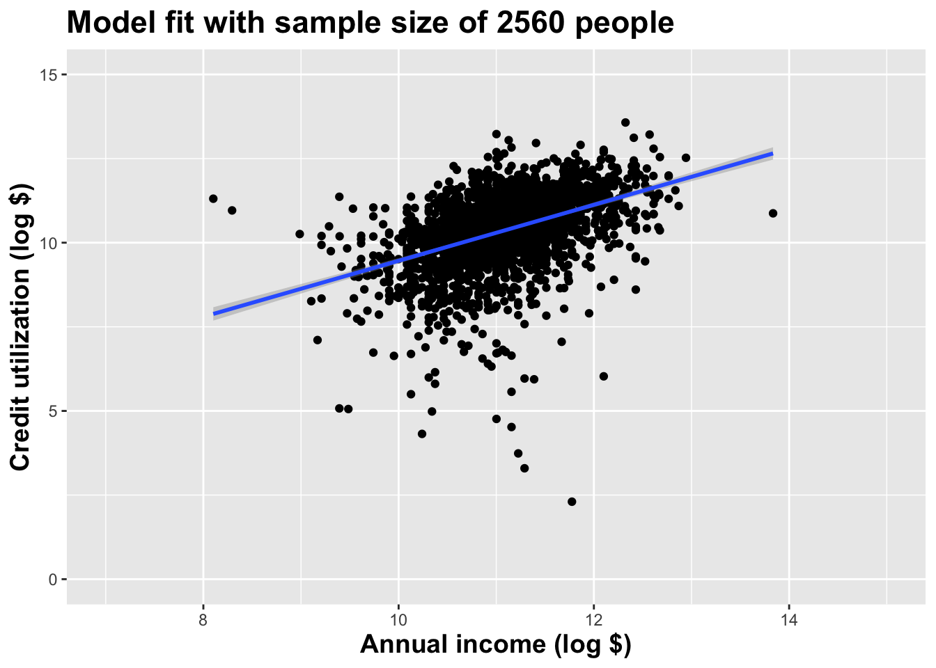
Double the sample size again
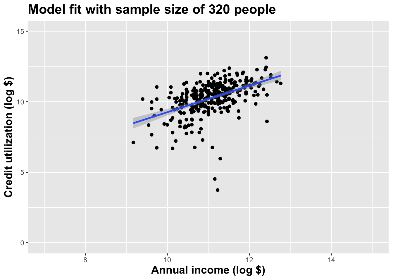
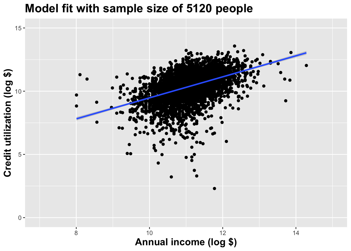
Double the sample size again
Double the sample size again
Double the sample size again
Double the sample size again
Double the sample size again
Double the sample size again
Double the sample size yet again
Double the sample size one more time
Use all the data we have
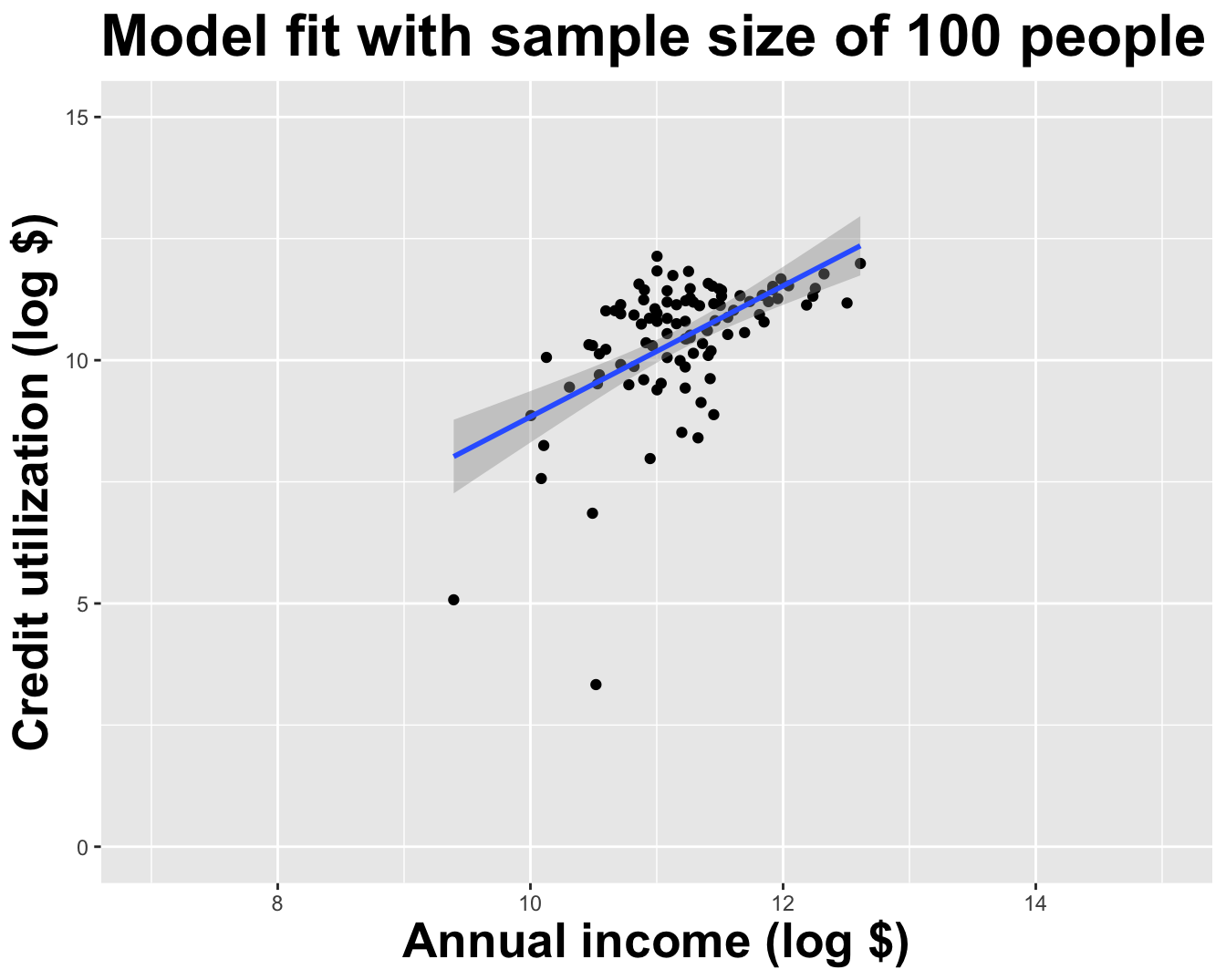
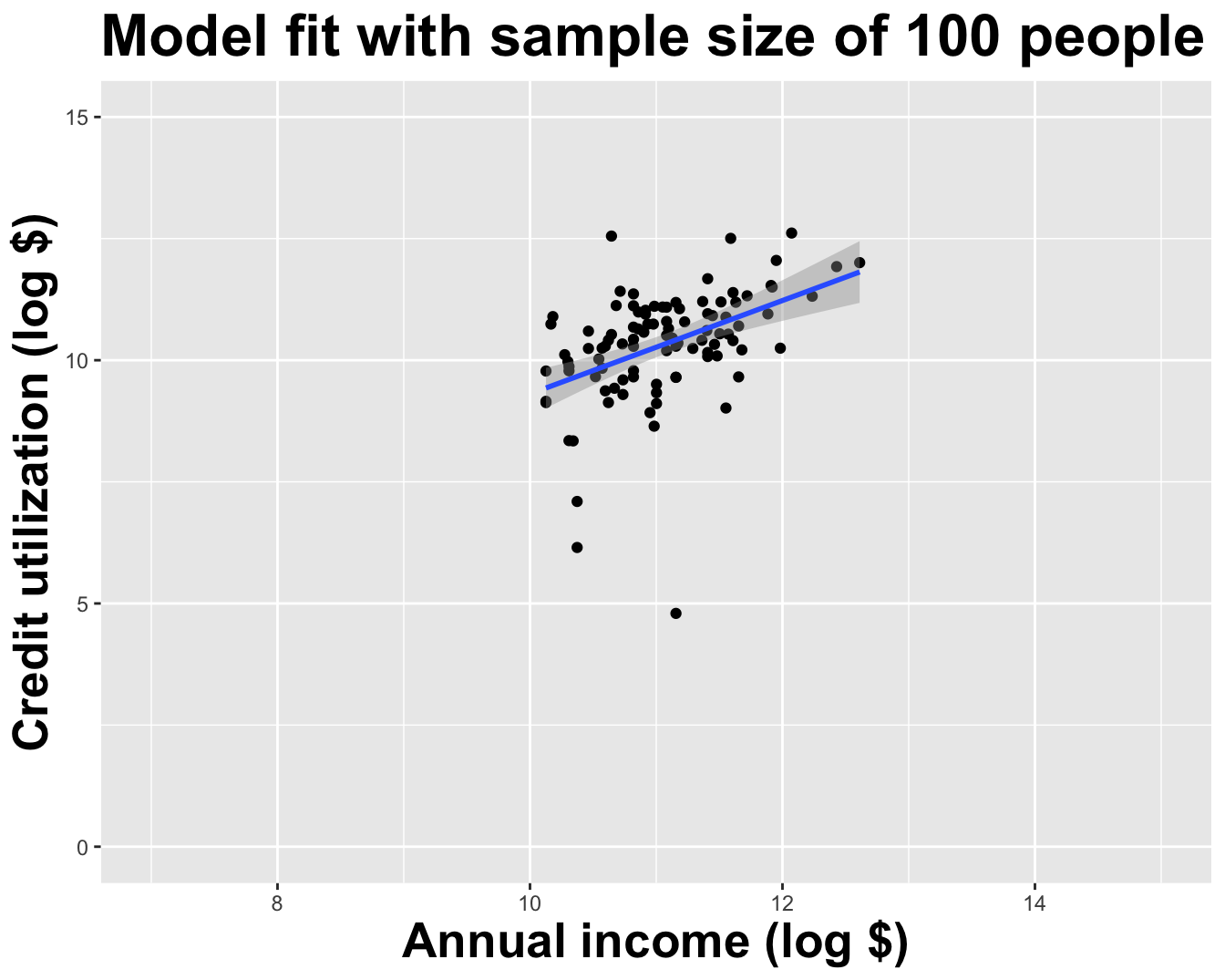
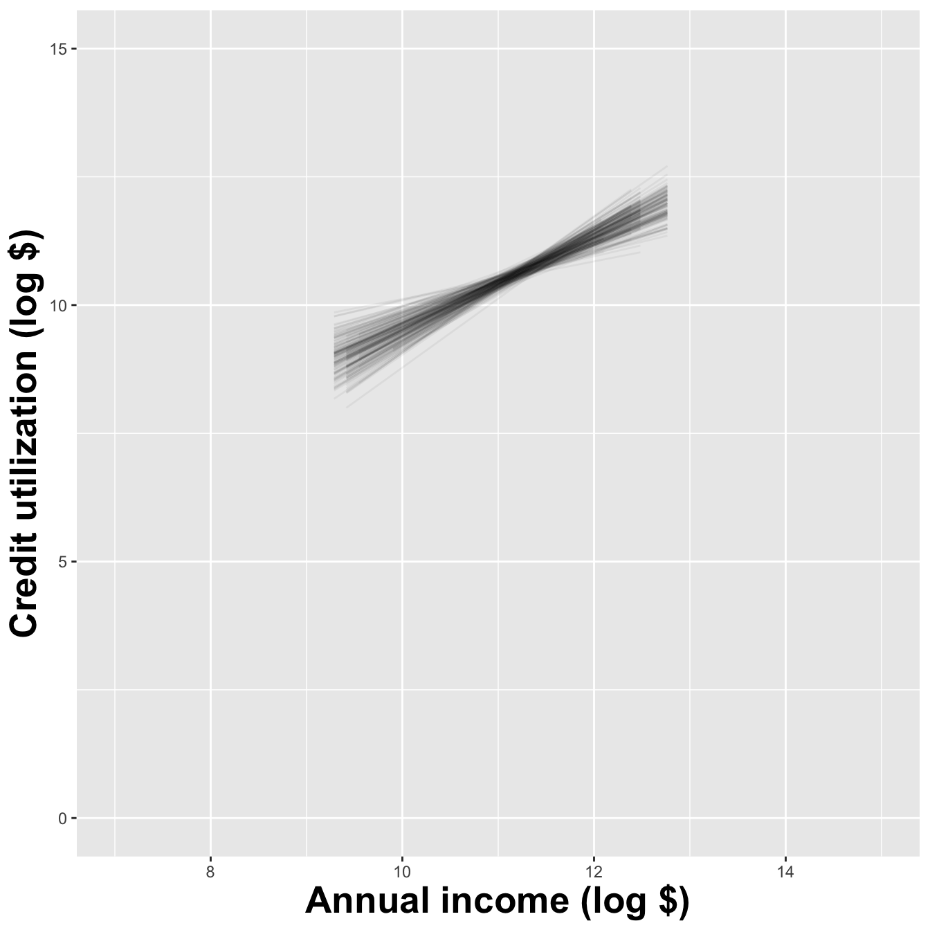
Here’s one dataset we could have seen
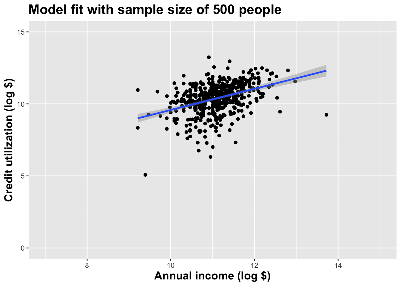
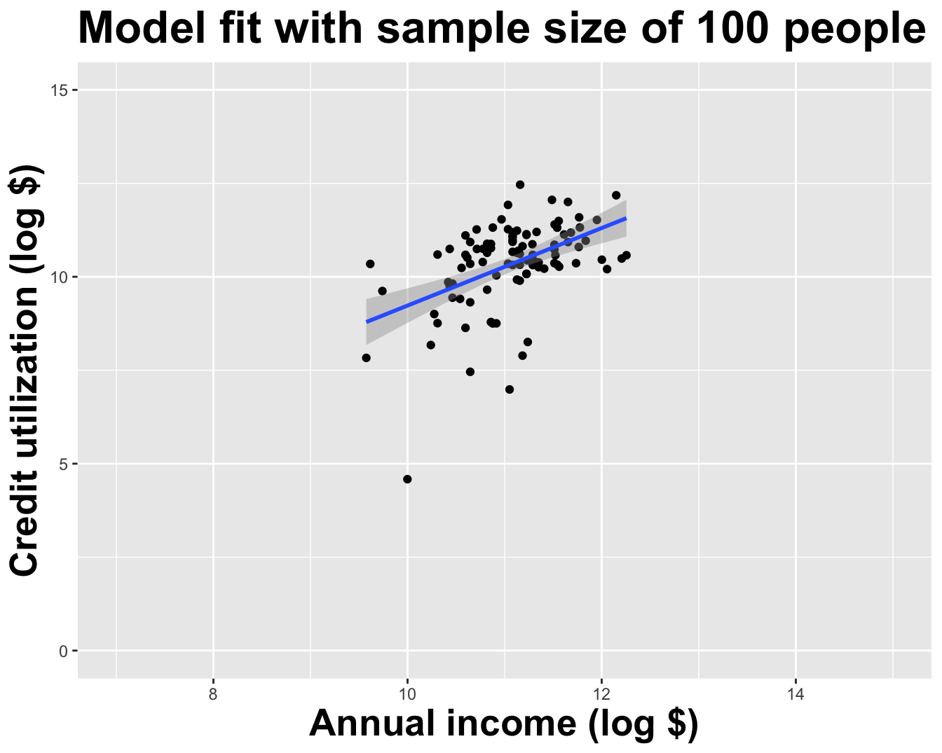
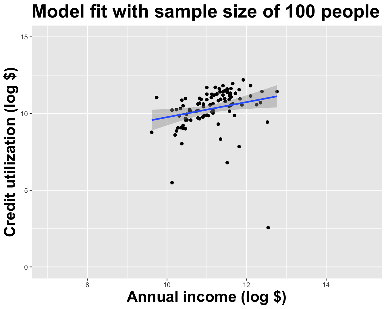
Here’s another
Here’s yet one more
Alternative 1
Alternative 2

Alternative 3
Different data set -> different estimates
# A tibble: 2 × 2
  term        estimate
  <chr>          <dbl>
1 (Intercept)    4.27
2 log_inc        0.553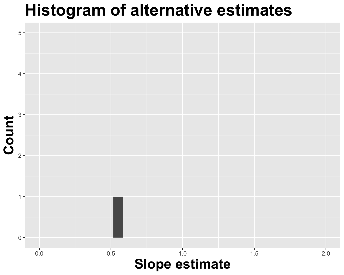
Different data set -> different estimates
# A tibble: 2 × 2
  term        estimate
  <chr>          <dbl>
1 (Intercept)    -4.63
2 log_inc         1.35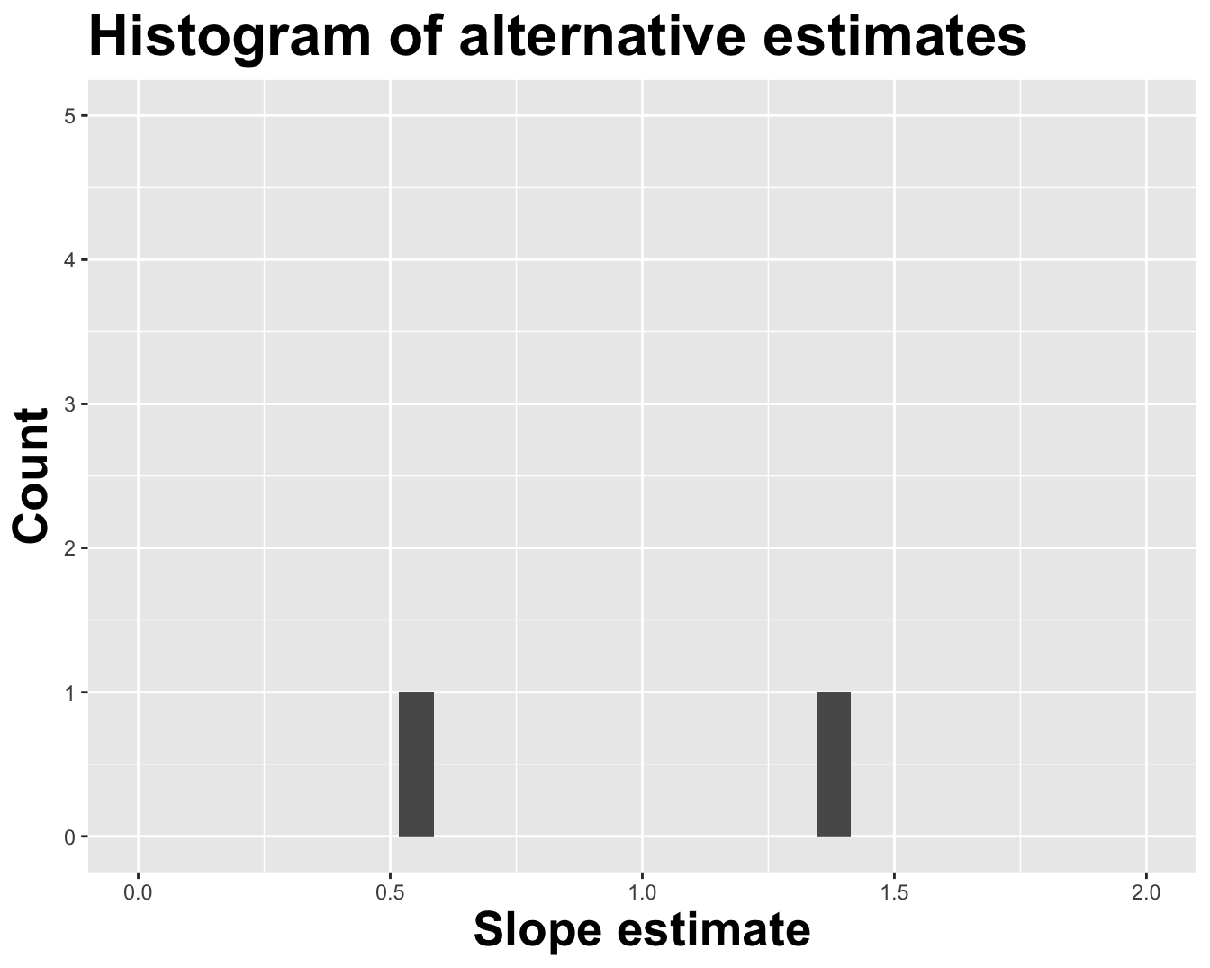
Different data set -> different estimates
# A tibble: 2 × 2
  term        estimate
  <chr>          <dbl>
1 (Intercept)    -1.14
2 log_inc         1.04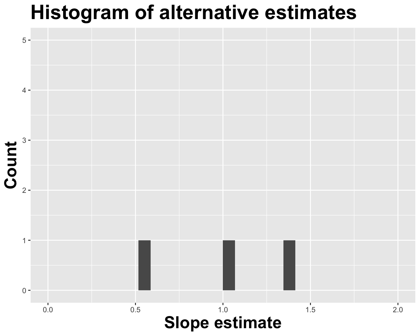
Different data set -> different estimates
# A tibble: 2 × 2
  term        estimate
  <chr>          <dbl>
1 (Intercept)   -0.288
2 log_inc        0.960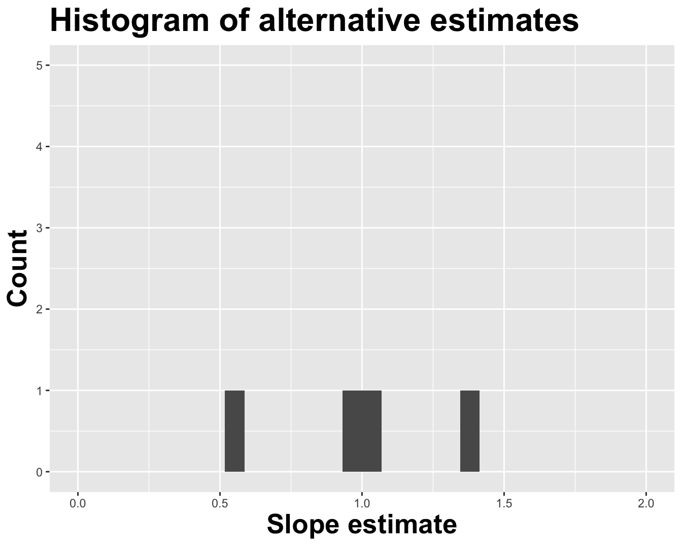
Different data set -> different estimates
# A tibble: 2 × 2
  term        estimate
  <chr>          <dbl>
1 (Intercept)    4.84
2 log_inc        0.492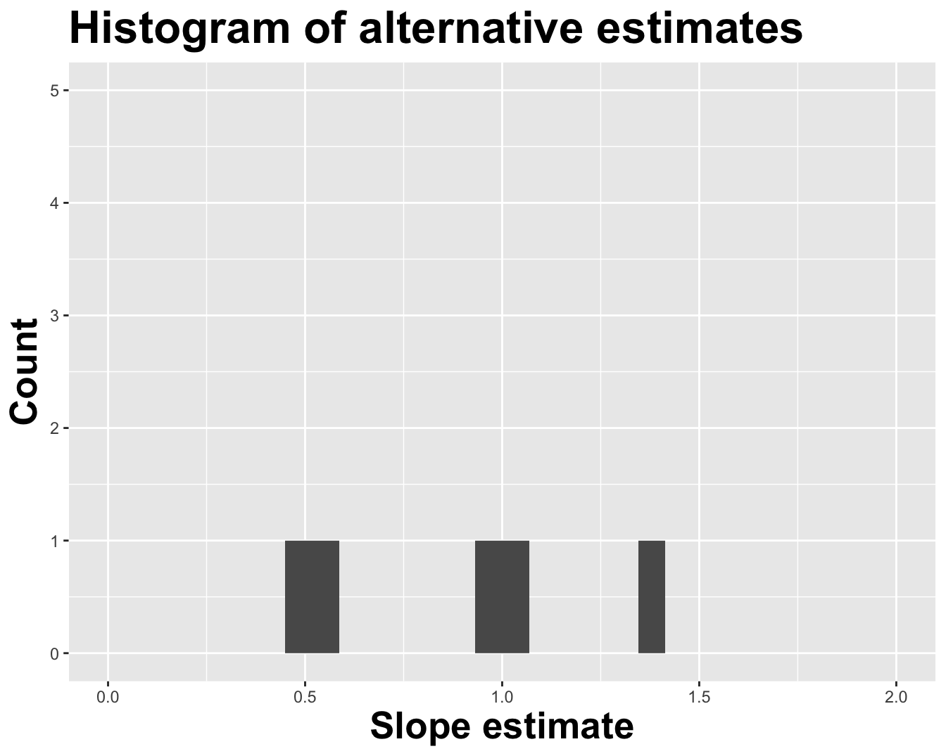
Different data set -> different estimates
# A tibble: 2 × 2
  term        estimate
  <chr>          <dbl>
1 (Intercept)    3.20
2 log_inc        0.654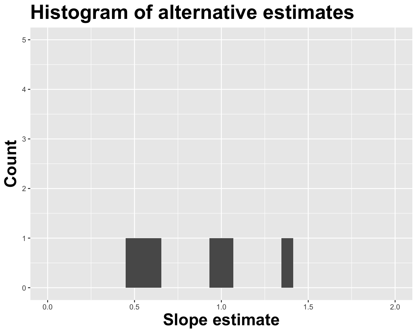
You get the idea

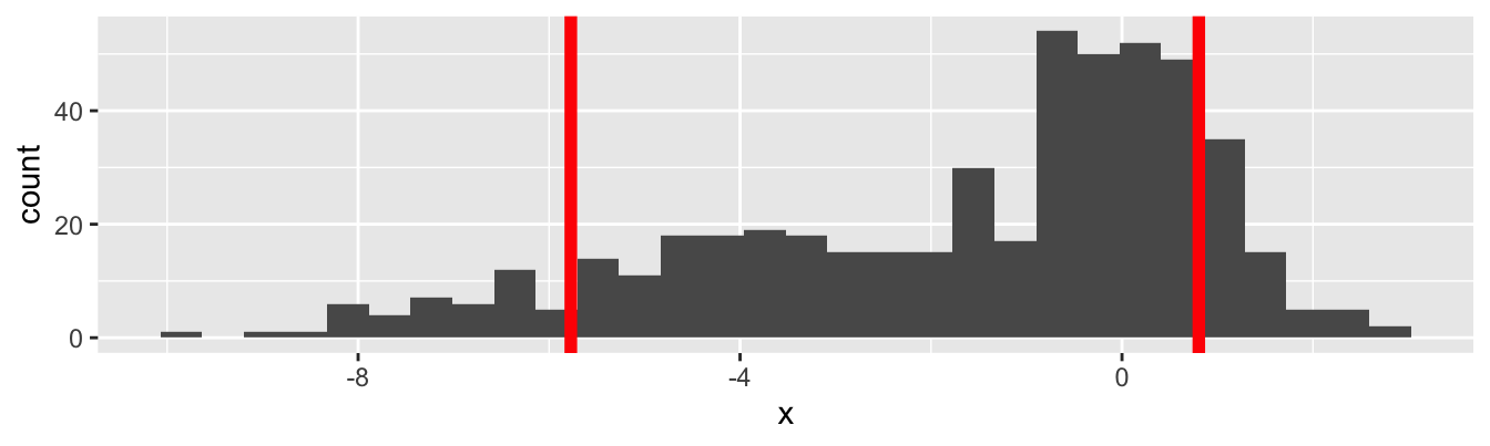
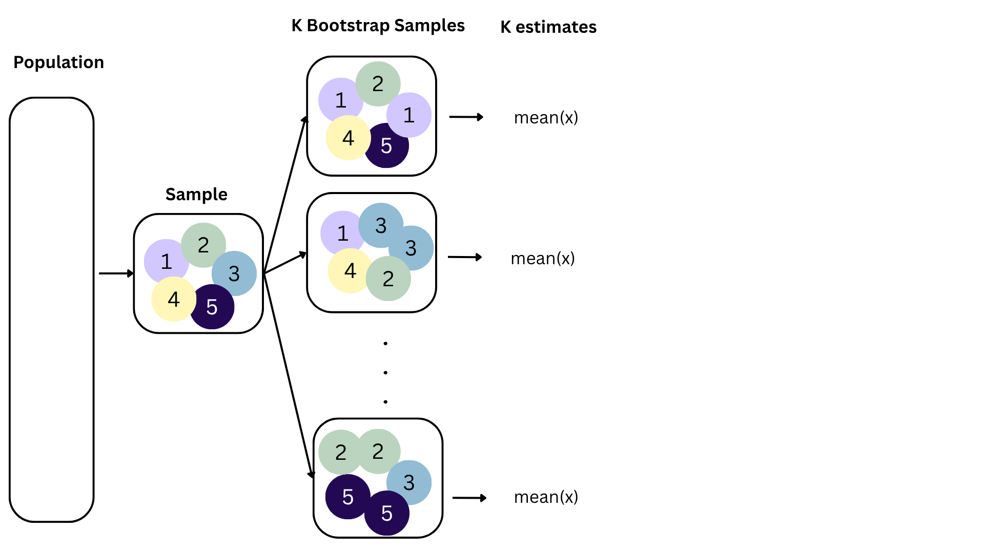
Variation in estimates across alternative datasets
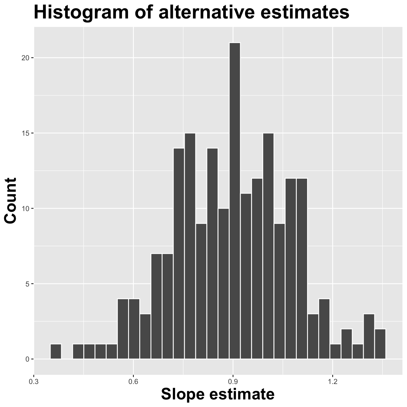
The amount of variation in the histogram tells us something about the uncertainty, and gives us a range of likely values.
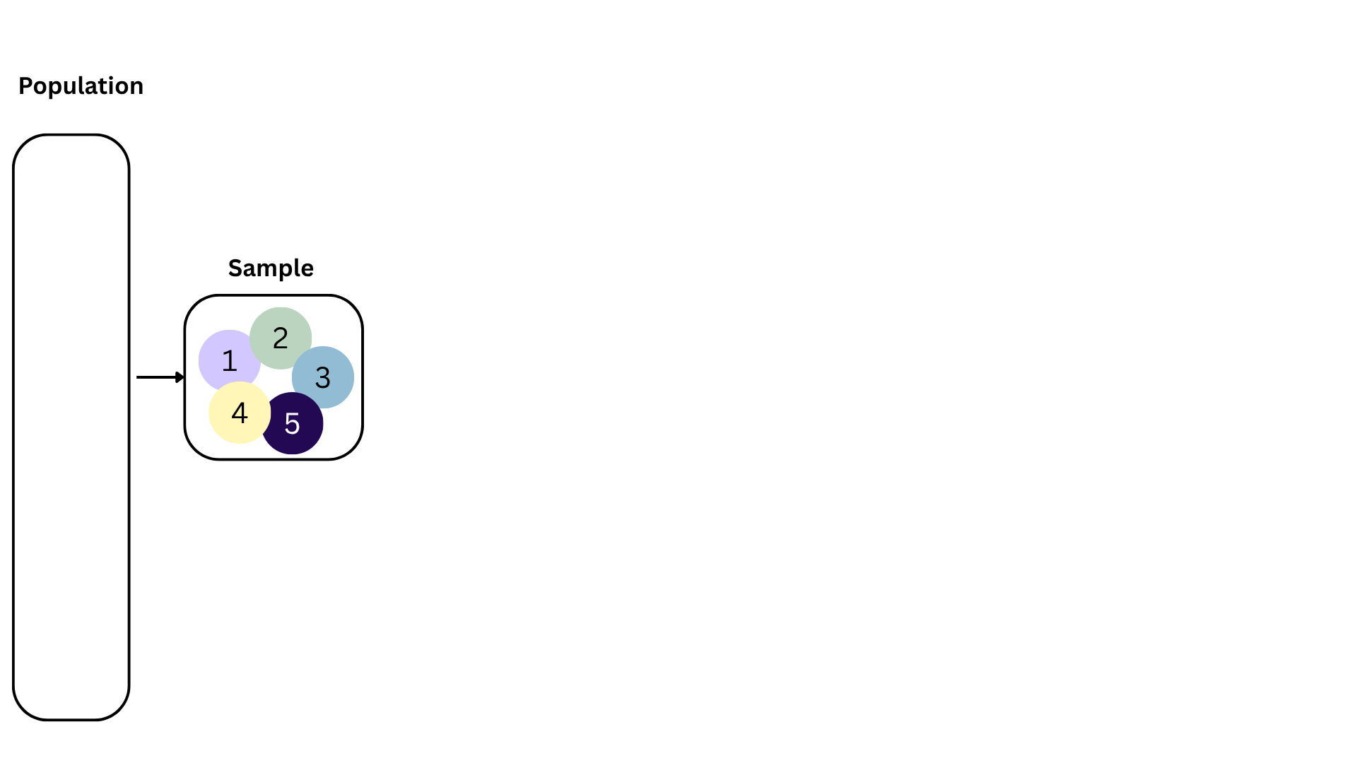
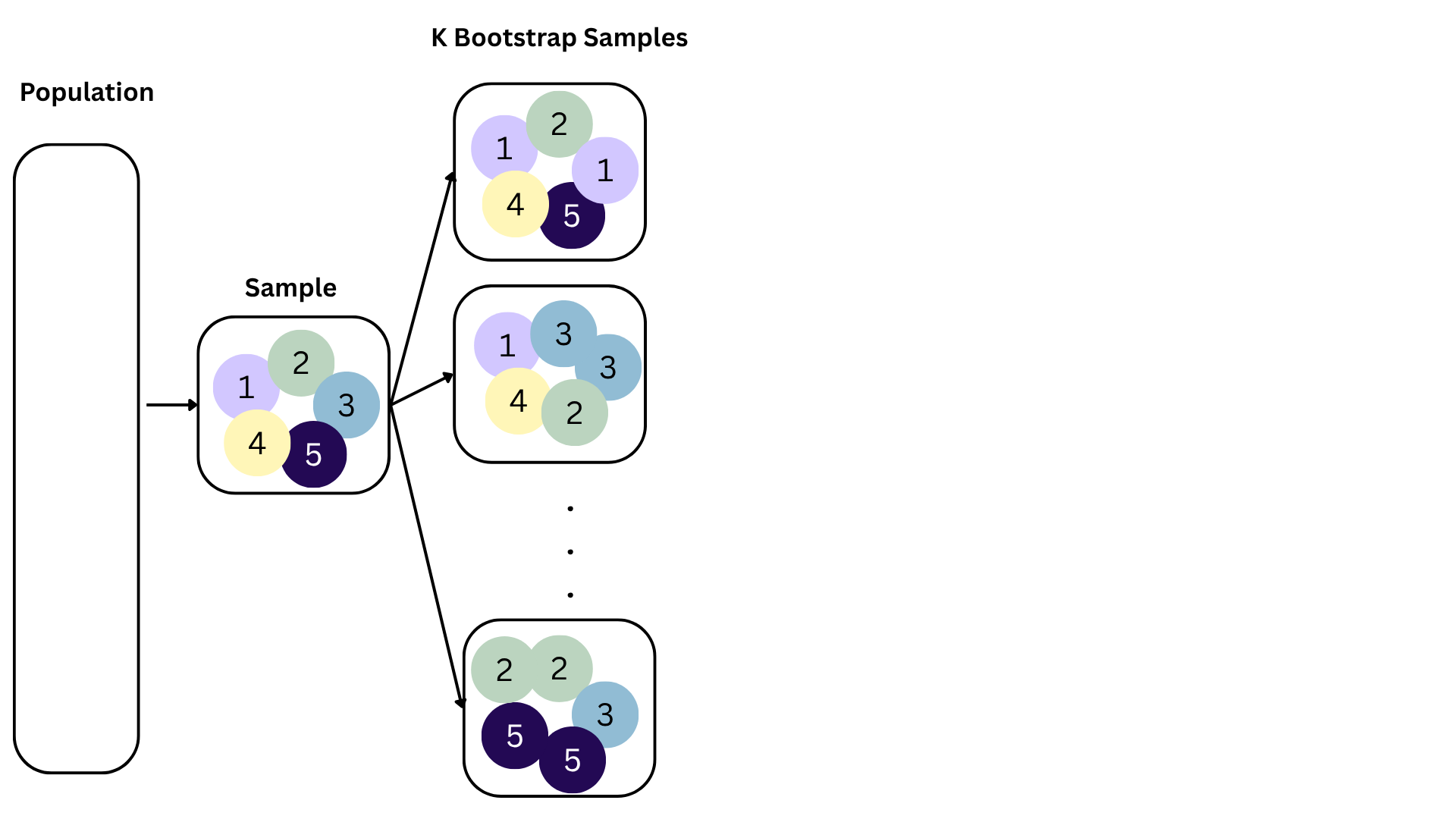
Bootstrapping
Bootstrapping
Bootstrapping
Bootstrapping
Bootstrapping
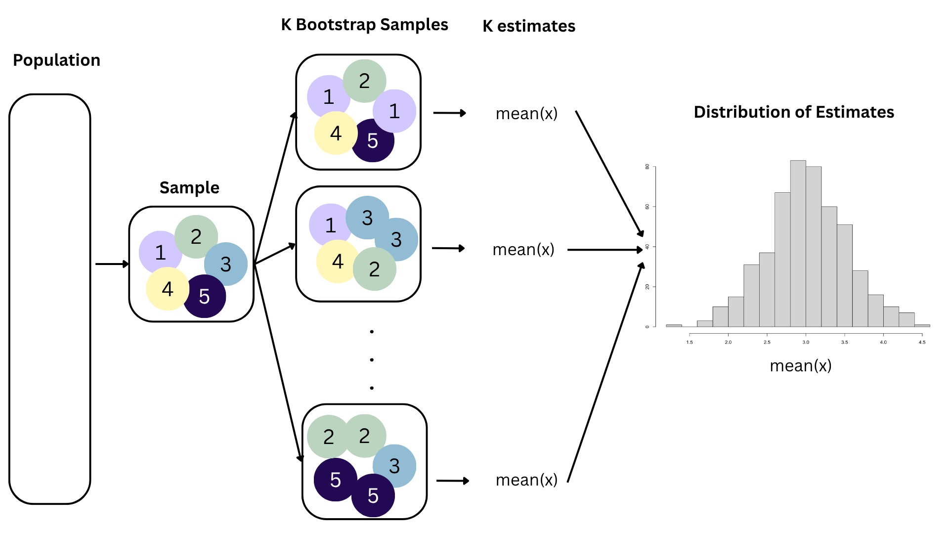
Bootstrapping
Bootstrapping
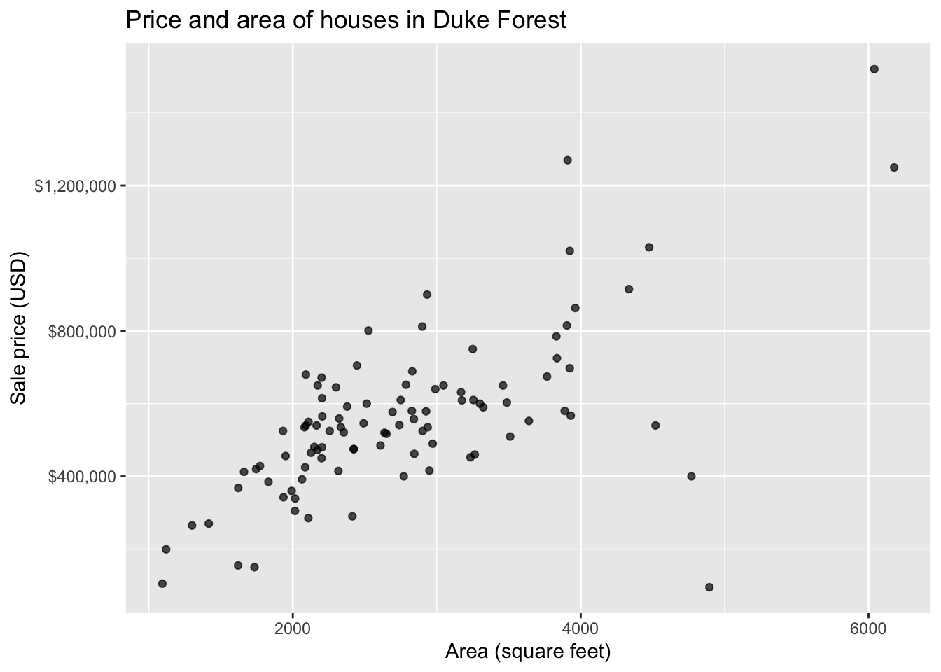
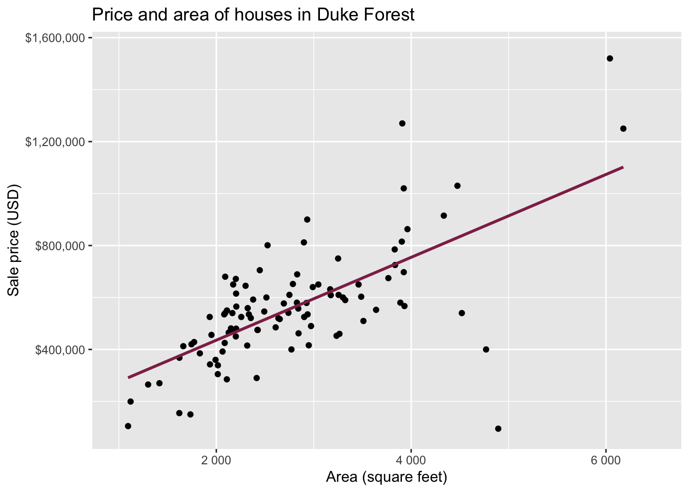
Data: Houses in Duke Forest
- Data on houses that were sold in the Duke Forest neighborhood of Durham, NC around November 2020
- Scraped from Zillow
- Source:
openintro::duke_forest

Goal: Use the area (in square feet) to understand variability in the price of houses in Duke Forest.
Exploratory data analysis
Statistical inference
Statistical inference provide methods and tools so we can use the single observed sample to make valid statements (inferences) about the population it comes from
For our inferences to be valid, the sample should be random and representative of the population we’re interested in

Bootstrap sample 1


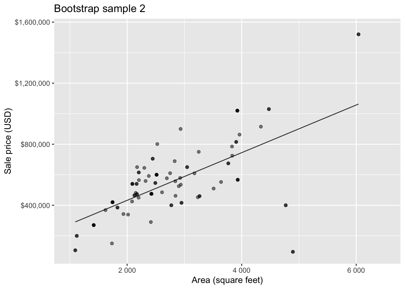
Bootstrap sample 2

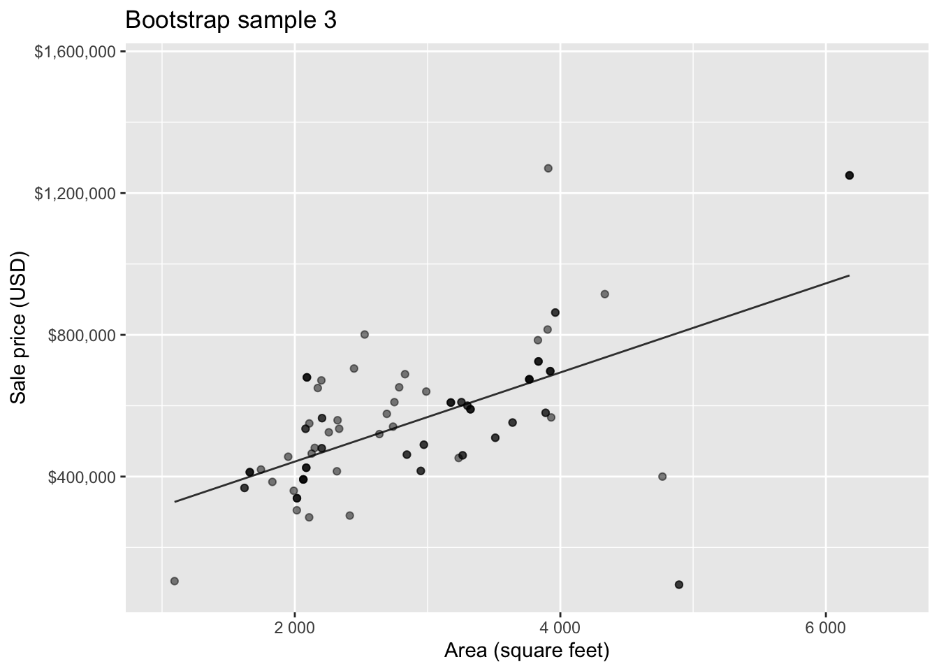
Bootstrap sample 3

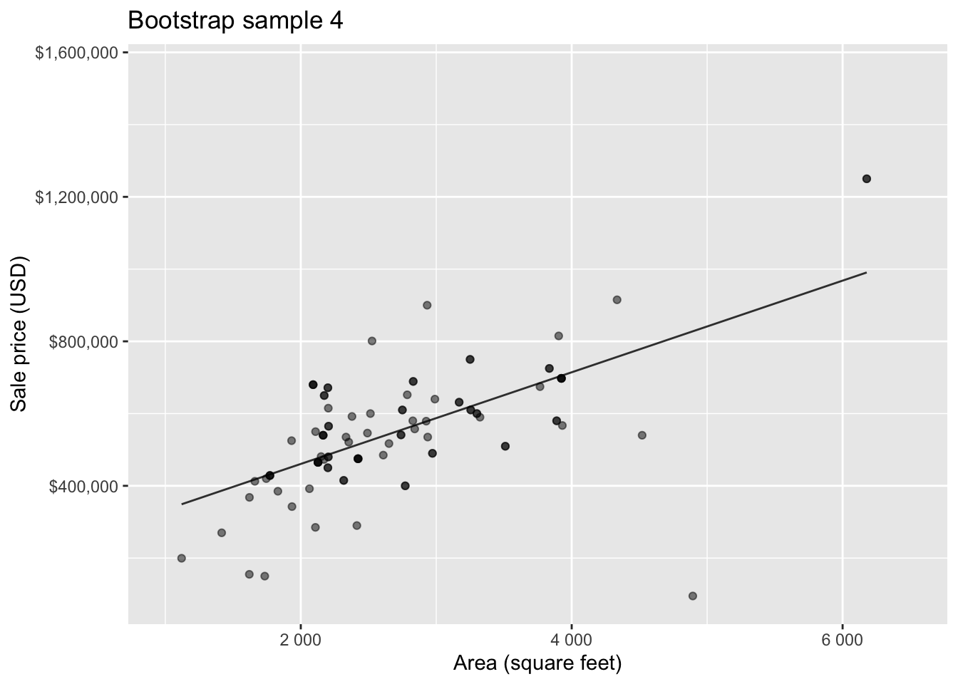
Bootstrap sample 4

Bootstrap sample 5
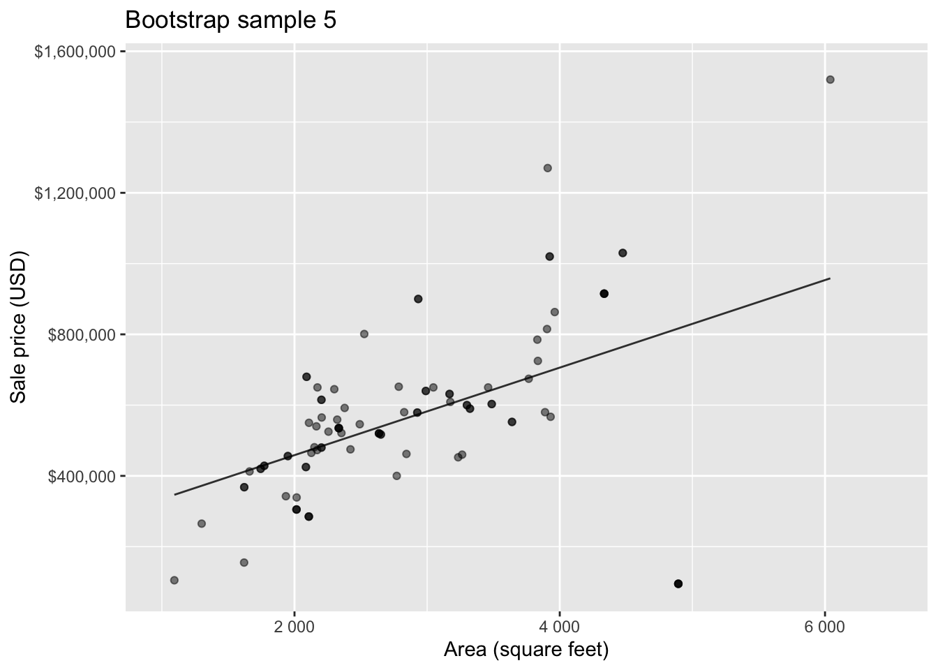
so on and so forth…
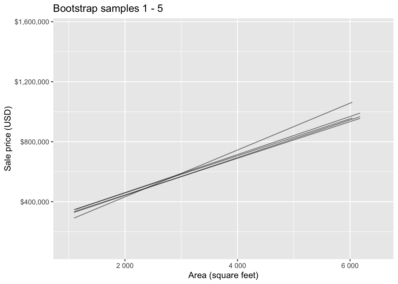
Bootstrap samples 1 - 5

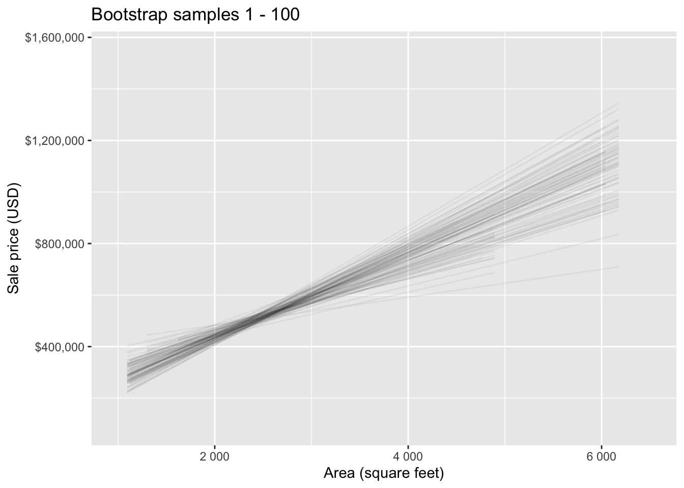
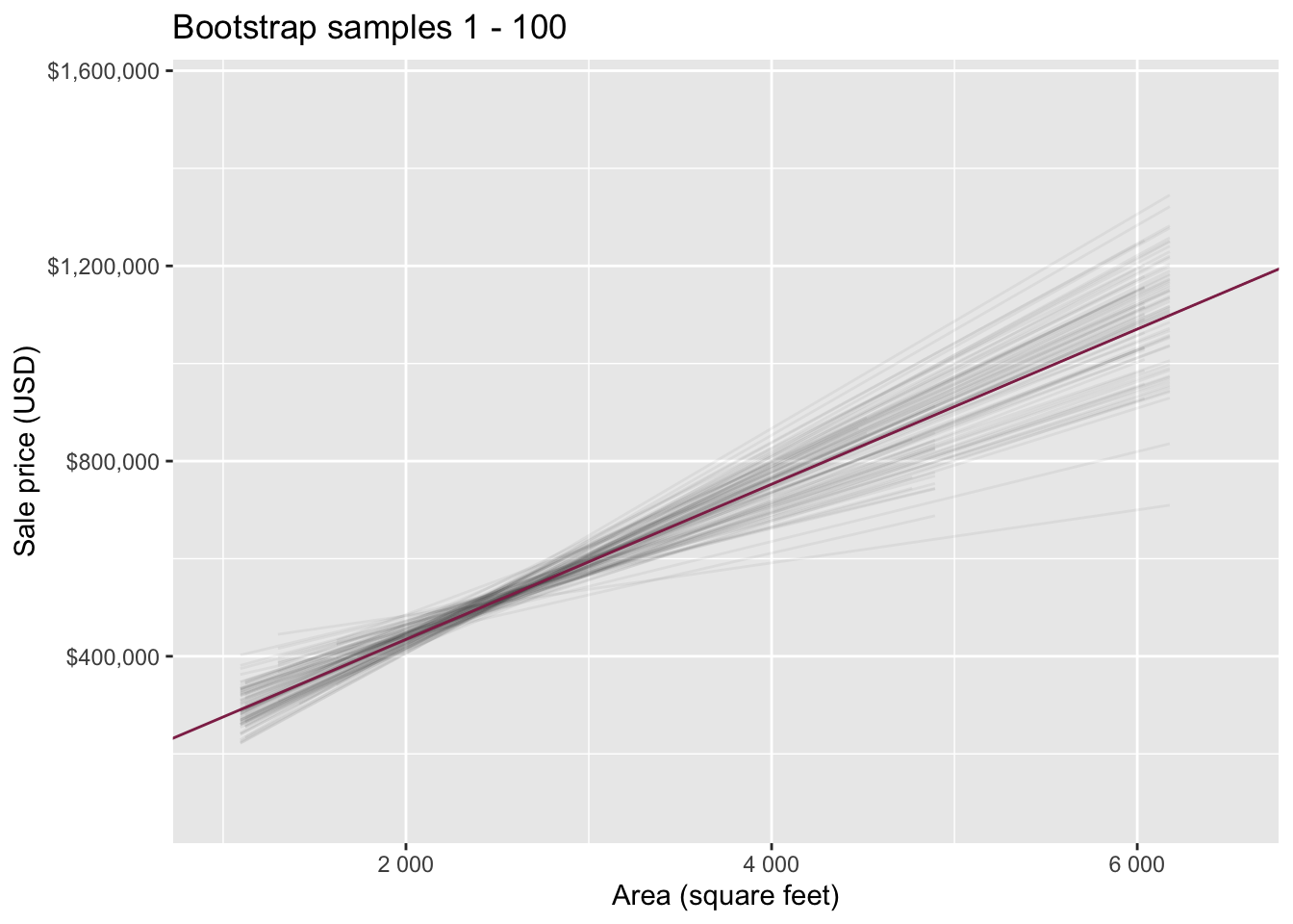
Bootstrap samples 1 - 100

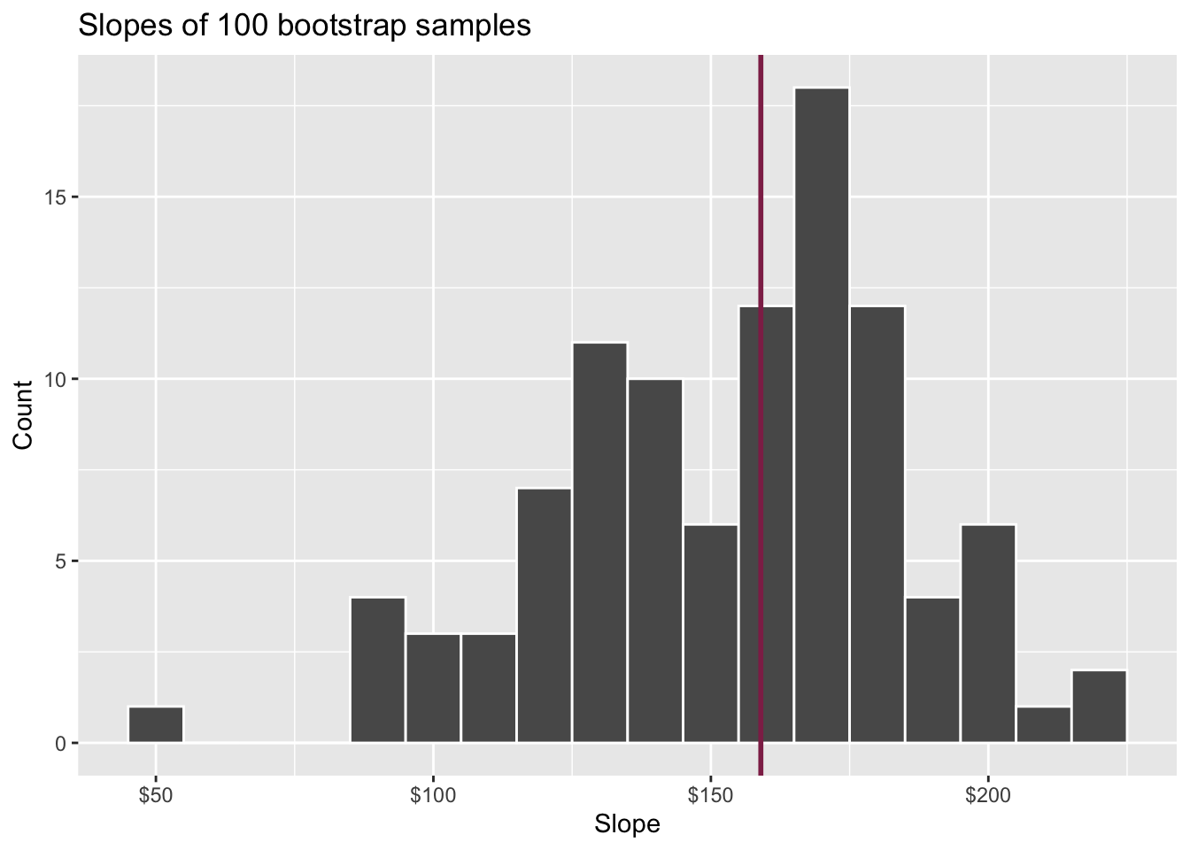
Slopes of bootstrap samples
Fill in the blank: For each additional square foot, the model predicts the sale price of Duke Forest houses to be higher, on average, by $159, plus or minus ___ dollars.
Slopes of bootstrap samples
Fill in the blank: For each additional square foot, we expect the sale price of Duke Forest houses to be higher, on average, by $159, plus or minus ___ dollars.

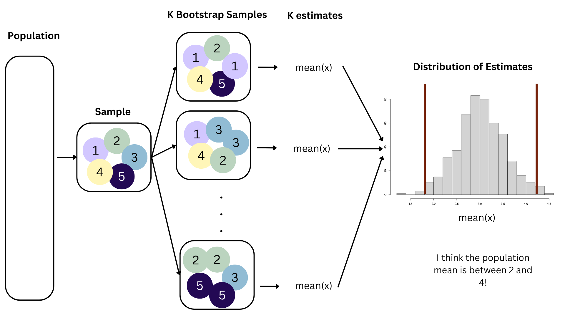
Confidence level
How confident are you that the true slope is between $0 and $250? How about $150 and $170? How about $90 and $210?
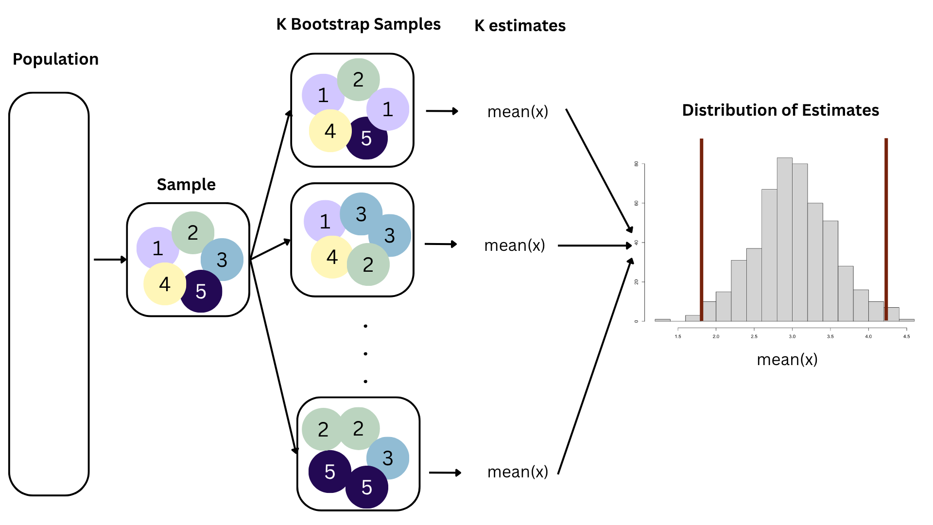
95% confidence interval
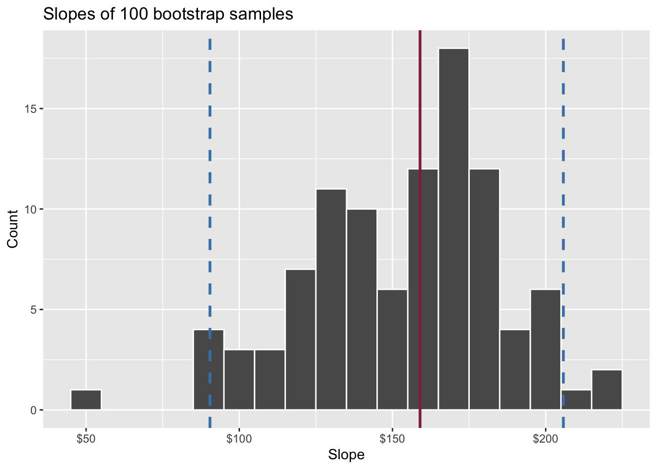
- A 95% confidence interval is bounded by the middle 95% of the bootstrap distribution
- We are 95% confident that for each additional square foot, the model predicts the sale price of Duke Forest houses to be higher, on average, by $90.43 to $205.77.
Precision vs. accuracy
If we want to be very certain that we capture the population parameter, should we use a wider or a narrower interval? What drawbacks are associated with using a wider interval?