Inference overview

Lecture 24

John Zito

Duke University
STA 199 Spring 2026

2026-04-20

While you wait: Participate 📱💻

What is a p-value?

The probability that the null hypothesis is true given your result.
The probability of a result as or more extreme than the one you got.
The probability of a result as or more extreme than the one you got assuming the null is true.
The probability that the alternative hypothesis is true given your result.
The probability that the null hypothesis and alternative hypothesis are both true given your result.

Scan the QR code or go HERE. Log in with your Duke NetID.

Chamber music tonight and tomorrow

April 20 @ 6PM (Nelson Music Room on East);
April 21 @ 7:30 PM (Baldwin);
Several past, present, and future(!) students;
Many bangers and bops, including JZ favorites by Ravel and Fauré.

Spread the word! Summer WANANA!

Summer Session 1
May 13 - June 25
Katie Solarz!

Summer Session 2
June 29 - August 10
Josh Lim!

Sorry gang

What the summer kids will get:

What you got:

The final exam

Monday May 1 @ 2pm in Griffith Theater
Make Testing Center appointments now!
Similar style and format to midterms
Longer than midterm, but shouldn’t take full 3 hours
Cumulative, with a bit more weight on the new inference stuff
As before, you get both sides of one 8.5” x 11” sheet of notes, prepared however you want.

Recap: statistical inference

The bottom line, at the top

Data science is the messy, real-world art of converting data into knowledge;
Statistics is the mathematical study of quantifying uncertainty about that knowledge to help guide decision-making.

The population model (greek letters, no hats)

This is an idealized representation of the data: \[ y = \beta_0+\beta_1x +\varepsilon; \]
There is some “true line” floating out there with a “true slope” \(\beta_1\) and “true intercept” \(\beta_0\);
With infinite amounts of perfectly measured data, we could know \(\beta_0\) and \(\beta_1\) exactly;
We don’t have that, so we must use finite amounts of imperfect data to estimate;
We are especially interested in \(\beta_1\) because is characterizes the association between \(x\) and \(y\), which is useful for prediction.

“Three branches of statistical government”

\(\beta_1\) is an unknown quantity we are trying to learn about using noisy, imperfect data. Learning comes in three flavors:

POINT ESTIMATION: get a single-number best guess for \(\beta_1\);
INTERVAL ESTIMATION: get a range of likely values for \(\beta_1\) that characterizes (sampling) uncertainty;
HYPOTHESIS TESTING: use the data to distinguish competing claims about \(\beta_1\).

Point estimation (roman letters, hats!)

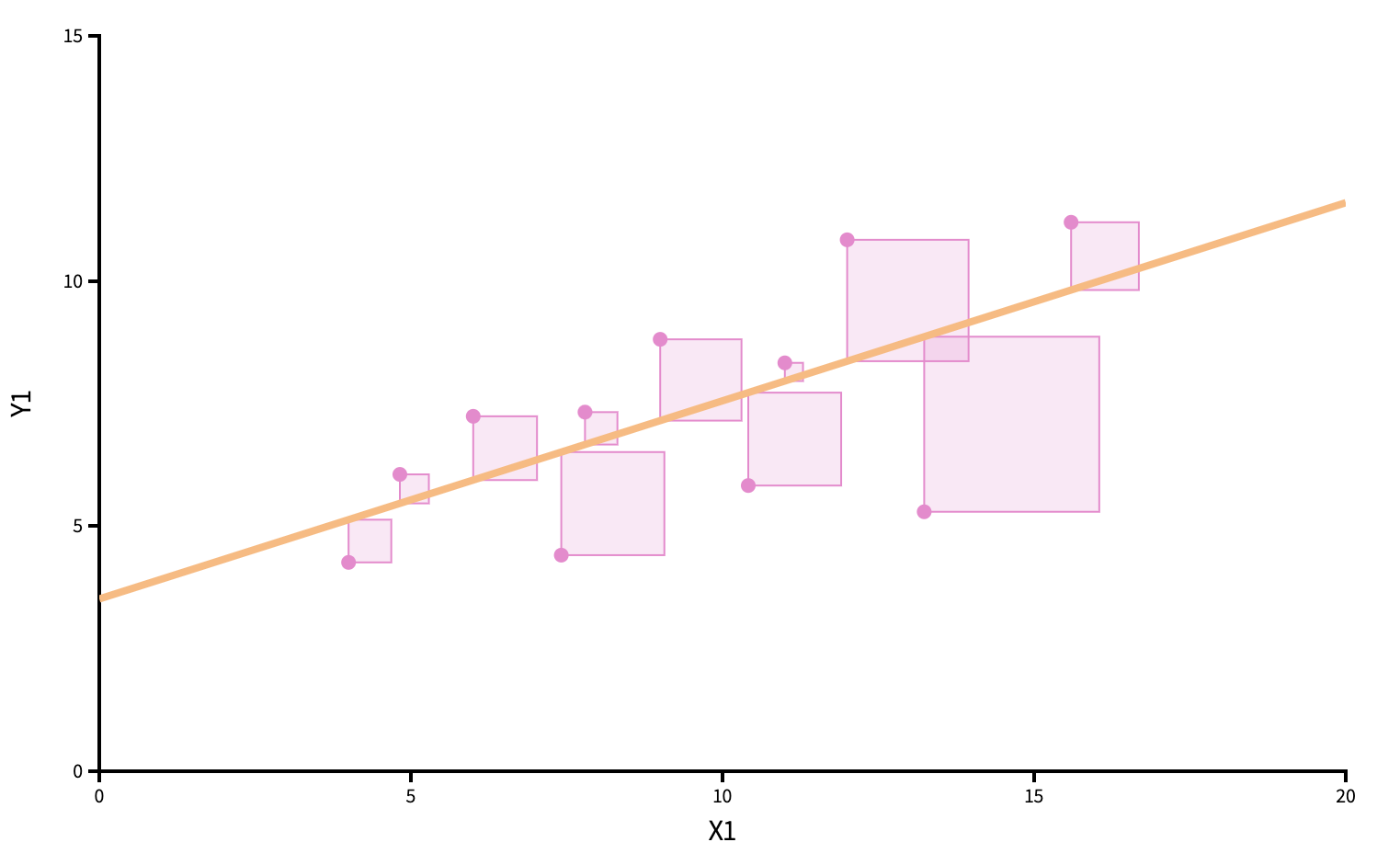
We estimate \(\beta_0\) and \(\beta_1\) with the coefficients of the best fit line:

\[ \hat{y}=b_0+b_1x. \]

“Best” means “least squares.” We pick the estimates so that the sum of squared residuals is as small as possible. Play around!

Point estimation

ggplot(mtcars, aes(x = wt, y = mpg)) + 
  geom_point() +
  geom_smooth(method = "lm")

Point estimation

linear_reg() |>
  fit(mpg ~ wt, data = mtcars) |>
  tidy()

# A tibble: 2 × 5
  term        estimate std.error statistic  p.value
  <chr>          <dbl>     <dbl>     <dbl>    <dbl>
1 (Intercept)    37.3      1.88      19.9  8.24e-19
2 wt             -5.34     0.559     -9.56 1.29e-10

Sampling uncertainty

How do our point estimates vary across alternative, hypothetical datasets?
- If they vary alot, uncertainty is high, and results are unreliable;
- if they vary only a little, uncertainty is low, and results are more reliable.
We can use the bootstrap to construct alternative datasets and assess the sensitivity of our estimates to changes in the data.

Bootstrap distribution

This histogram displays variation in the slope estimate across alternative datasets.

Large spread >> high uncertainty;
Small spread >> lower uncertainty.

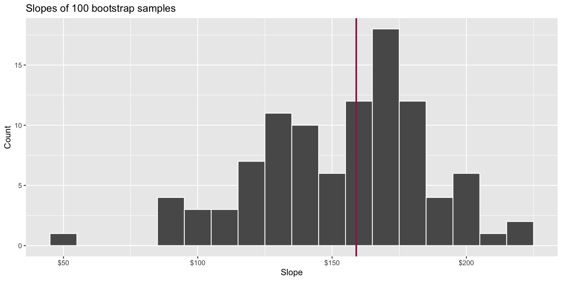
Confidence interval

Pick a range that swallows up a large % of the histogram:

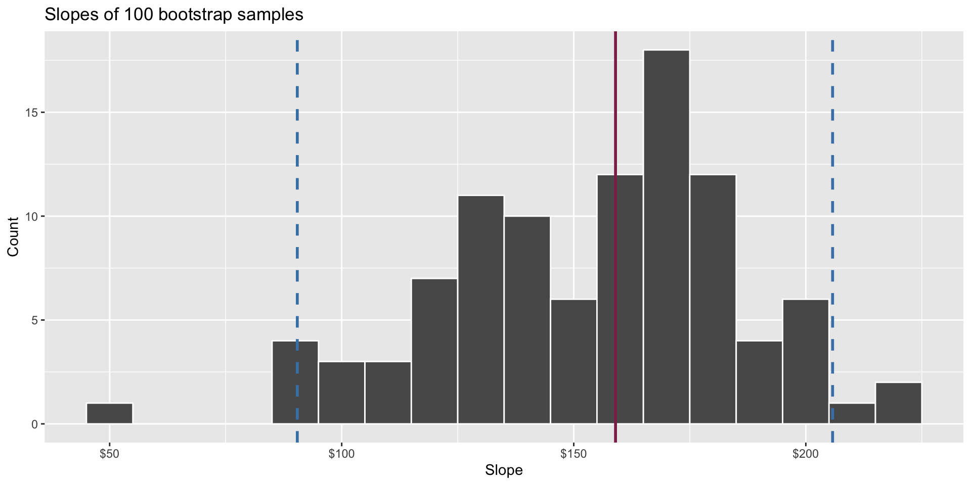
We use quantiles (think IQR) but there are other ways.

Hypothesis testing

Two competing claims about \(\beta_1\): \[ \begin{aligned} H_0&: \beta_1=0\quad(\text{nothing going on})\\ H_A&: \beta_1\neq0\quad(\text{something going on}) \end{aligned} \]
Do the data strongly favor one or the other?
How can we quantify this?

Hypothesis testing

Think hypothetically: if the null hypothesis were in fact true, would my results be out of the ordinary?
- if no, then the null could be true;
- if yes, then the null might be bogus;
My results represent the reality of actual data. If they conflict with the null, then you throw out the null and stick with reality;
How do we quantify “would my results be out of the ordinary”?

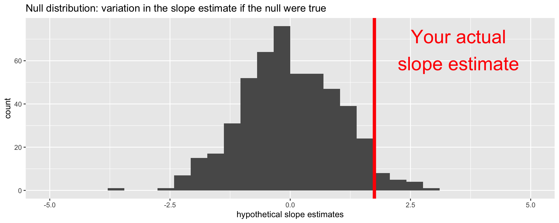
Null distribution

If the null happened to be true, how would we expect our results to vary across datasets? We can use simulation to answer this:

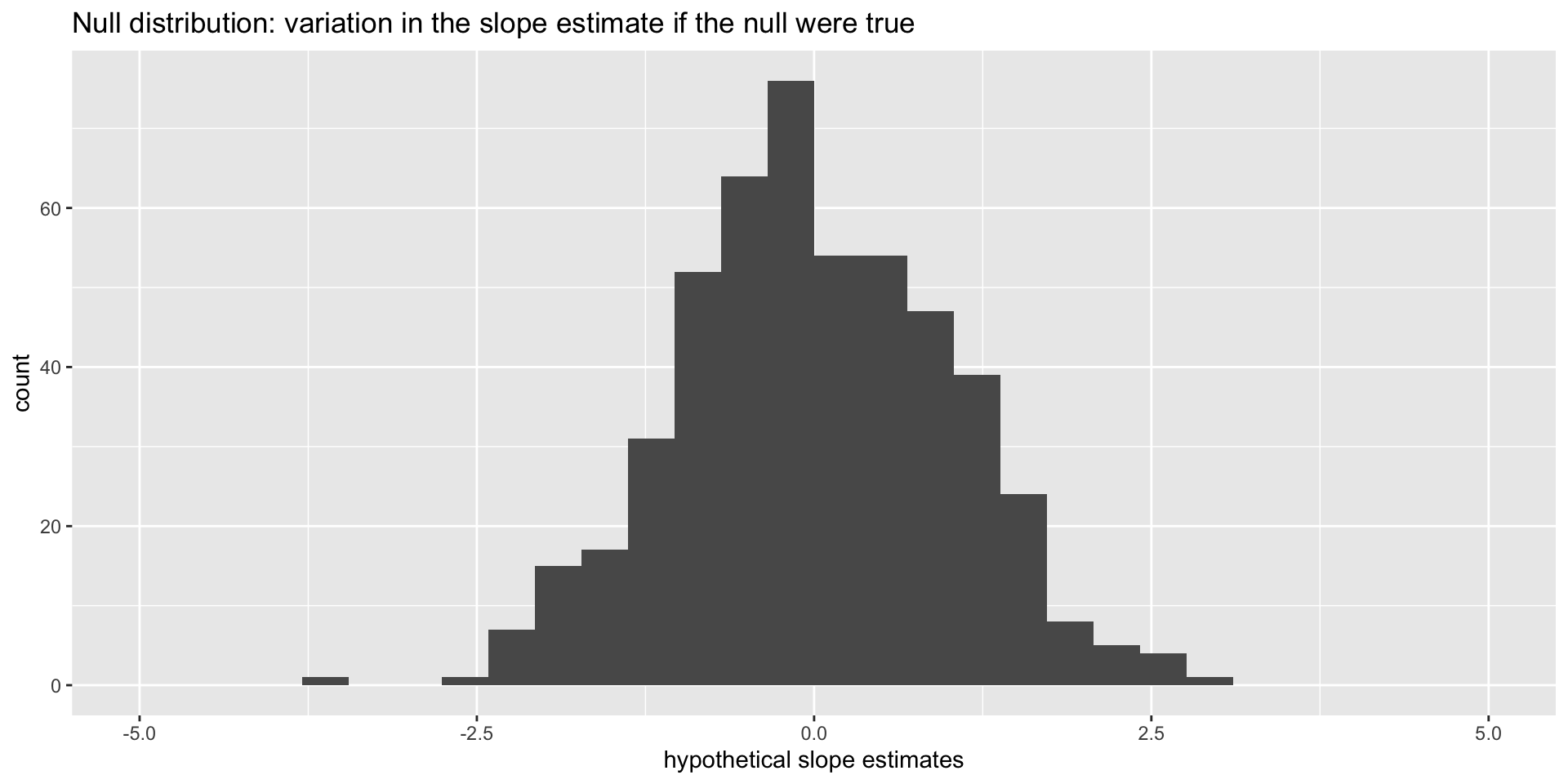
This is how the world should look if the null is true.

Null distribution versus reality

Locate the actual results of your actual data analysis under the null distribution. Are they in the middle? Are they in the tails?

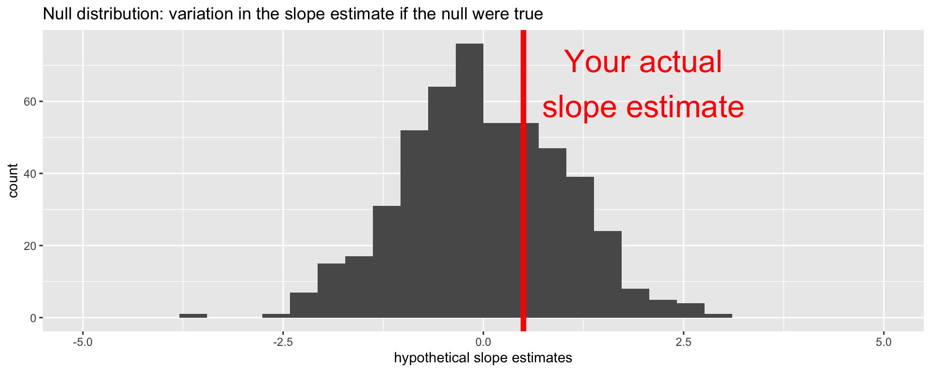
Are these results in harmony or conflict with the null?

Null distribution versus reality

Locate the actual results of your actual data analysis under the null distribution. Are they in the middle? Are they in the tails?

Are these results in harmony or conflict with the null?

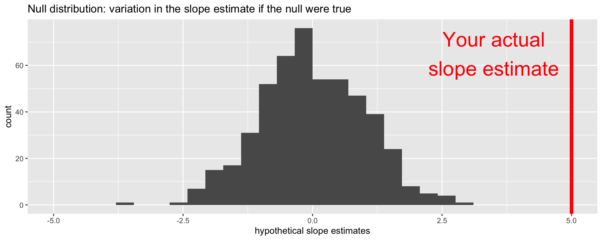
Null distribution versus reality

Locate the actual results of your actual data analysis under the null distribution. Are they in the middle? Are they in the tails?

Are these results in harmony or conflict with the null?

The main idea

The point estimate is reality. That’s what the data say;
The null distribution is hypothetical;
Are the reality and the hypothetical in harmony or conflict?
- If harmony, the null remains plausible and cannot be dismissed;
- If conflict, go with reality (reject the null).
Instead of eyeballing a picture, how can we quantity the degree of “harmoniousness” between reality and the hypothetical?

p-value

The \(p\)-value is the probability of being even farther out in the tails of the null distribution than your results already were.

if this number is very low, then your results would be out of the ordinary if the null were true, so maybe the null was never true to begin with;
if this number is high, then your results may be perfectly compatible with the null.

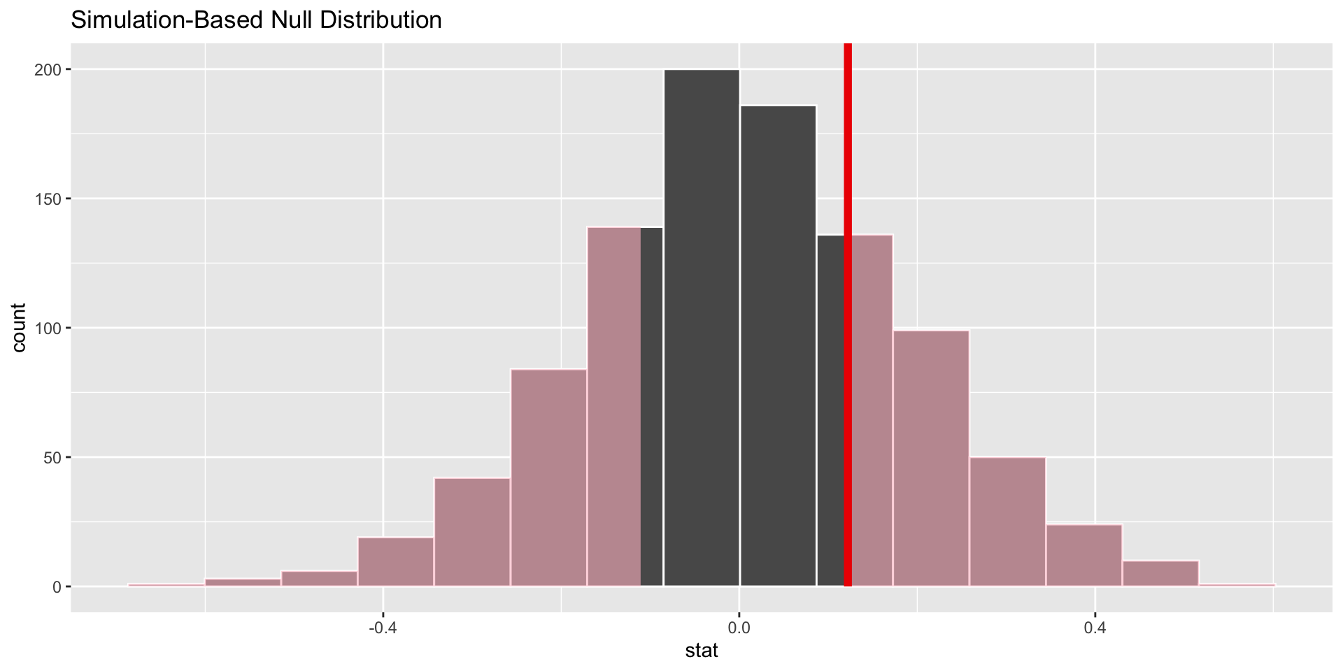
p-value

p-value is the fraction of the histogram area shaded red:

Big ol’ p-value. Null remains plausible

p-value

p-value is the fraction of the histogram area shaded red:

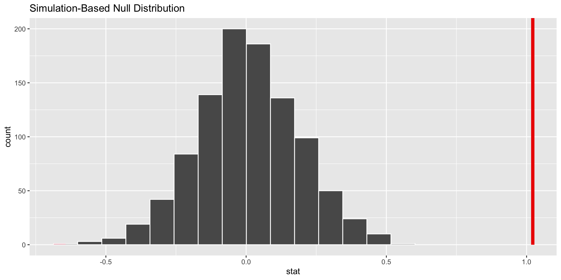
p-value is basically zero. Null looks bogus.

p-value

p-value is the fraction of the histogram area shaded red:

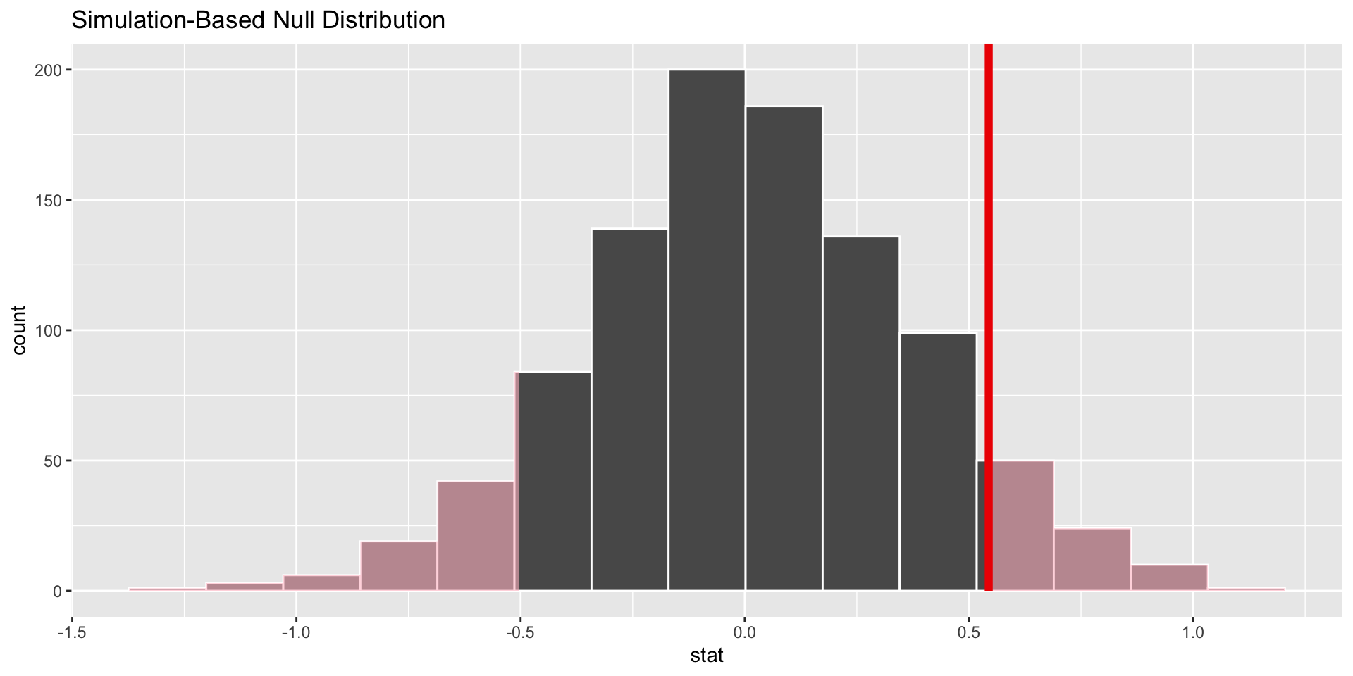
p-value is…kinda small? Null looks…?

Discernibility level

How do we decide if the p-value is big enough or small enough?
Pick a threshold \(\alpha\in[0,\,1]\) called the discernibility level:
- If \(p\text{-value} < \alpha\), reject null and accept alternative;
- If \(p\text{-value} \geq \alpha\), fail to reject null;
Standard choices: \(\alpha=0.01, 0.05, 0.1, 0.15\).

Wooclap-a-palooza

Get in there

Scan the QR code or go HERE. Log in with your Duke NetID.

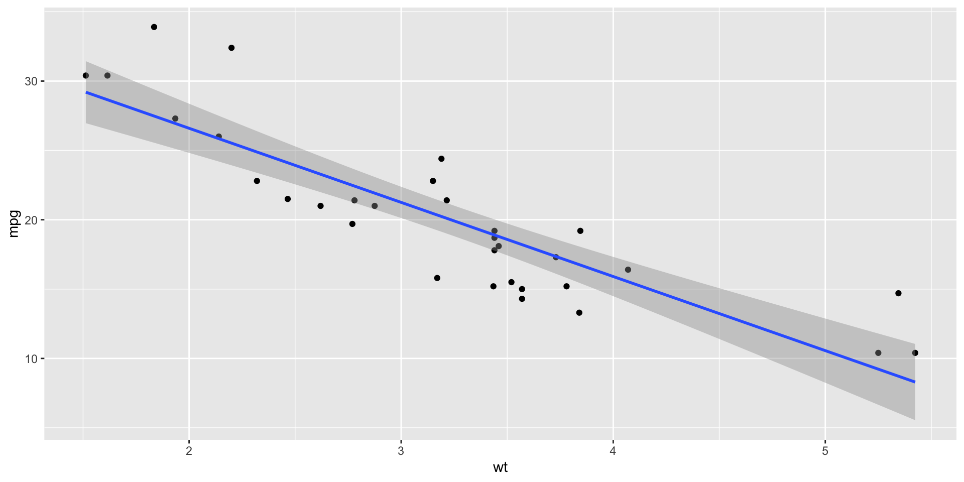
What is \(b_1\)?

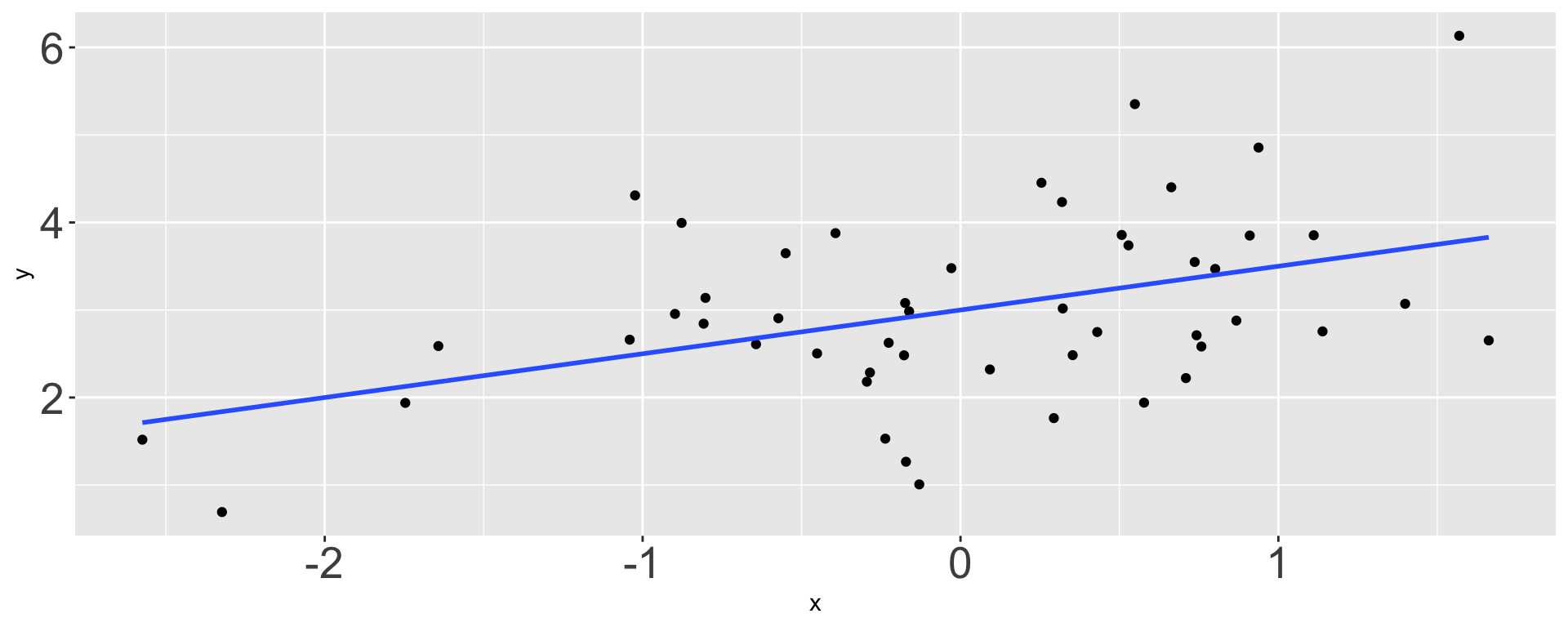
-1 / 2
0
1 / 4

1 / 2
1
2

What is \(b_0\)?

1
1.75

Which of these could be a bootstrap sample?

This is the original dataset:

Rows: 5
Columns: 1
$ scores <dbl> 1.563, -0.515, 1.206, -0.411, 0.523

A	B	C	D
-0.515	1.563	-0.515	-0.522
-0.411	-0.411	-0.411	1.12
1.563	-0.515	-0.411	1.206
-0.515		1.563	0.68
-0.515		1.563	0.83
		0.523
		1.563

Which is a 98% confidence interval?

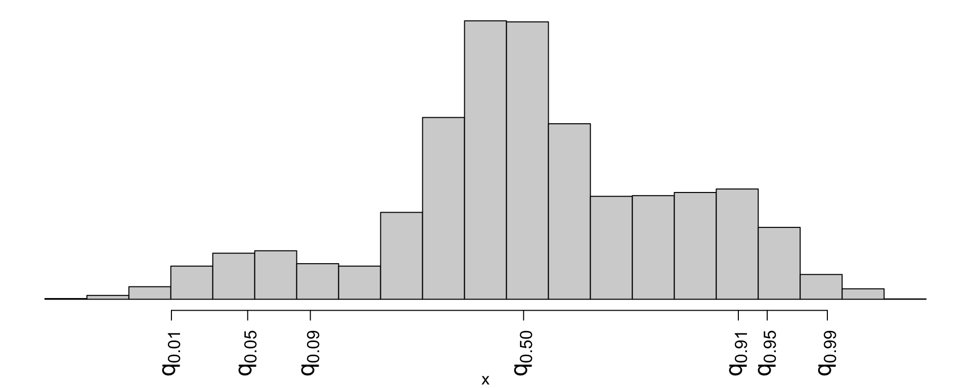
\((q_{0.01},\,q_{0.91})\)
\((q_{0.01},\,q_{0.99})\)

\((q_{0.09},\,q_{0.95})\)
\((q_{0.05},\,q_{0.99})\)

Match the picture to the p-value.

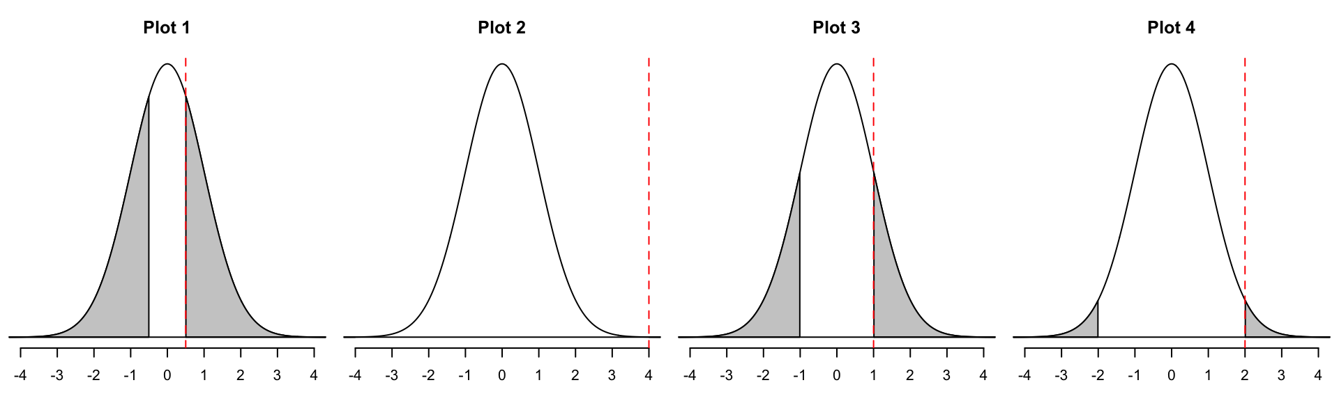
0
0.045

0.32
0.62

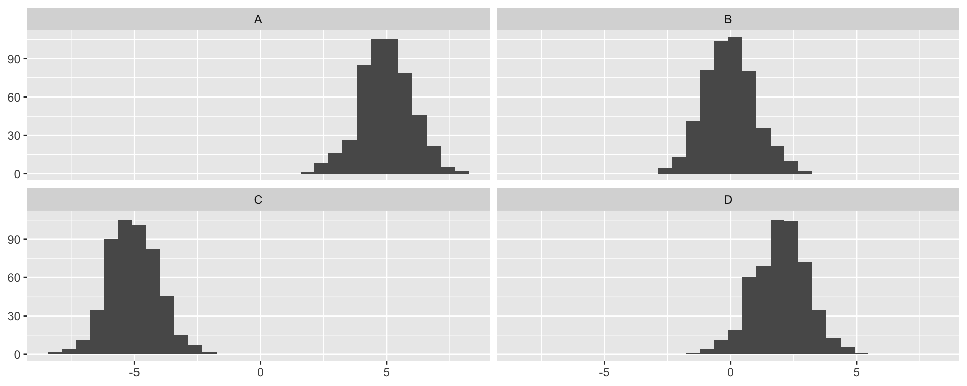
Which could be the null distribution of the test?

For these hypotheses

\[ \begin{aligned} H_0&: \beta_1=5\\ H_A&: \beta_1\neq 5. \end{aligned} \]

Application exercise

ae-24-card-krueger

Go to your ae project in RStudio.
If you haven’t yet done so, make sure all of your changes up to this point are committed and pushed, i.e., there’s nothing left in your Git pane.
If you haven’t yet done so, click Pull to get today’s application exercise file: ae-24-card-krueger.qmd.
Work through the application exercise in class, and render, commit, and push your edits.