AE 03: Bechdel + data visualization

In this mini-analysis, we use the data from the FiveThirtyEight story “The Dollar-And-Cents Case Against Hollywood’s Exclusion of Women.”

This analysis is about the Bechdel test, a measure of the representation of women in fiction.

Getting started

Packages

We’ll use the tidyverse package for this analysis.

library(tidyverse)

Data

The data are stored as a CSV (comma-separated values) file in your repository’s data folder. Let’s read it from there and save it as an object called bechdel.

bechdel <- read_csv("data/bechdel.csv")

Get to know the data

We can use the glimpse() function to get an overview (or “glimpse”) of the data.

glimpse(bechdel)

Rows: 1,615
Columns: 7
$ title       <chr> "21 & Over", "Dredd 3D", "12 Years a Slave", "2 Guns", "42…
$ year        <dbl> 2013, 2012, 2013, 2013, 2013, 2013, 2013, 2013, 2013, 2013…
$ gross_2013  <dbl> 67878146, 55078343, 211714070, 208105475, 190040426, 18416…
$ budget_2013 <dbl> 13000000, 45658735, 20000000, 61000000, 40000000, 22500000…
$ roi         <dbl> 5.221396, 1.206305, 10.585703, 3.411565, 4.751011, 0.81851…
$ binary      <chr> "FAIL", "PASS", "FAIL", "FAIL", "FAIL", "FAIL", "FAIL", "P…
$ clean_test  <chr> "notalk", "ok", "notalk", "notalk", "men", "men", "notalk"…

What does each observation (row) in the data set represent?

Each observation represents a film.

How many observations (rows) are in the data set?

There are 1615 movies in the dataset.

How many variables (columns) are in the data set?

There are 7 columns in the dataset.

Variables of interest

The variables we’ll focus on are the following:

gross_2013: how much did the movie earn at the box office (in 2013 $);
budget_2013: how much did the movie cost to make (in 2013 $);
roi: Return on investment, calculated as the ratio of the gross to budget;
- If the movie broke even, roi is 1;
- If the movie made money, roi is greater than 1;
- If the movie lost money, roi is between 0 and 1;
clean_test: Bechdel test result:
- ok = passes test
- dubious (Chinatown?)
- men = women only talk about men
- notalk = women don’t talk to each other
- nowomen = fewer than two women
binary: Bechdel Test PASS vs FAIL binary

We will also use the year of release in data prep and title of movie to take a deeper look at some outliers.

Film finances

How are budgets distributed?

Visualize the distribution of film budgets in the dataset:

ggplot(bechdel, aes(x = budget_2013)) + 
  geom_histogram() + 
  labs(x = "2013 USD",
       title = "Film budgets (1990 - 2013)")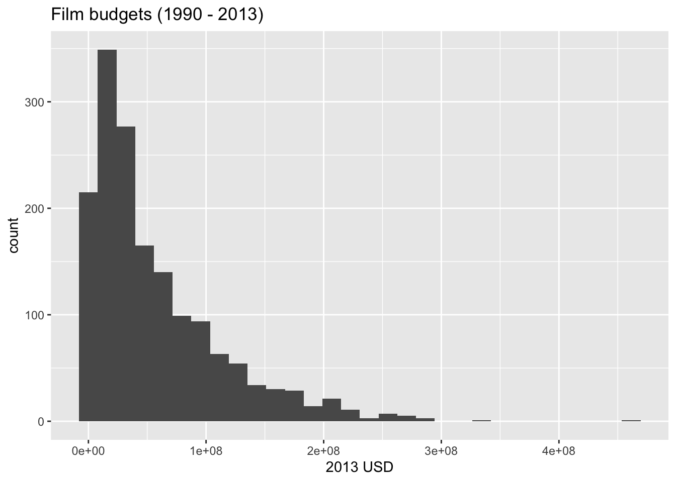

shape: right skewed;
center: the mean budget is about $57,035,015.00;
spread: the standard deviation is $55,976,978.00;
modality: unimodal (one peak);

How are budget and earnings related?

Visualize the relationship between a film’s budget and its earnings:

ggplot(bechdel, aes(x = budget_2013, y = gross_2013)) + 
  geom_point() + 
  geom_smooth() + 
  labs(x = "Budget (2013 USD)",
       y = "Gross (2013 USD)",
       title = "Film finances (1990 - 2013)")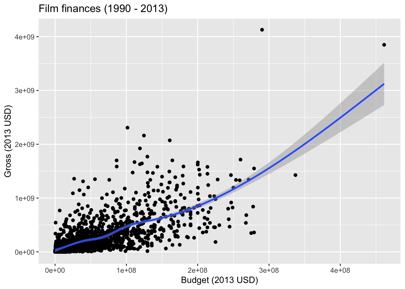

direction: positive;
shape: linear (the curve seems to be introduced only by the outliers in the upper right);
strength: moderate;

Which films are “outliers” in terms of gross?

bechdel |> 
  filter(gross_2013 > 3e9)

# A tibble: 2 × 7
  title    year gross_2013 budget_2013   roi binary clean_test
  <chr>   <dbl>      <dbl>       <dbl> <dbl> <chr>  <chr>     
1 Avatar   2009 3848295959   461435929  8.34 FAIL   men       
2 Titanic  1997 4127821329   290247625 14.2  PASS   ok

Bechdel test results

Visualizing data with ggplot2

ggplot2 is the package and ggplot() is the function in this package that is used to create a plot.

ggplot() creates the initial base coordinate system, and we will add layers to that base. We first specify the data set we will use with data = bechdel.

ggplot(data = bechdel)

The mapping argument is paired with an aesthetic (aes()), which tells us how the variables in our data set should be mapped to the visual properties of the graph.

ggplot(data = bechdel, mapping = aes(x = clean_test))

As we previously mentioned, we often omit the names of the first two arguments in R functions. So you’ll often see this written as:

ggplot(bechdel, aes(x = clean_test))

Note that the result is exactly the same.

The geom_xx function specifies the type of plot we want to use to represent the data. In the code below, we use geom_bar which allows us to see the frequency of each type of film in our dataset.

ggplot(bechdel, aes(x = clean_test)) +
  geom_bar()

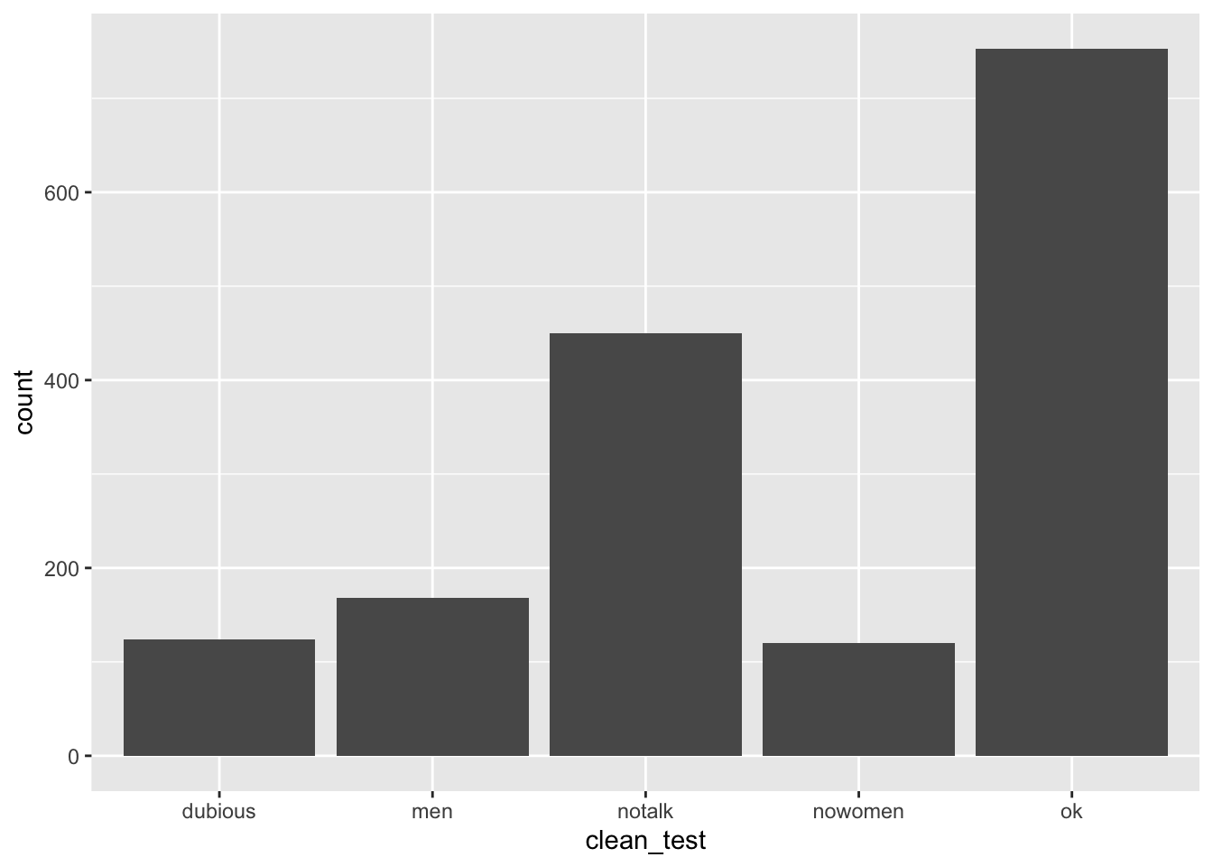
What types of movies are more common, those that pass or do not pass the test?

Render, commit, and push

Render your Quarto document.
Go to the Git pane and check the box next to each file listed, i.e., stage your changes. Commit your staged changes using a simple and informative message.
Click on push (the green arrow) to push your changes to your application exercise repo on GitHub.
Go to your repo on GitHub and confirm that you can see the updated files. Once your updated files are in your repo on GitHub, you’re good to go!

Return-on-investment

Let’s take a look at return-on-investment (ROI) for movies that do and do not pass the Bechdel test.

Step 1 - Your turn

Create side-by-side box plots of roi by clean_test where the boxes are colored by binary.

ggplot(bechdel, aes(x = clean_test, y = roi, color = binary)) +
  geom_boxplot() +
  labs(
    title = "Return on investment vs. Bechdel test result",
    x = "Detailed Bechdel result",
    y = "Return-on-investment (gross / budget)",
    color = "Bechdel\nresult"
  )

Warning: Removed 15 rows containing non-finite outside the scale range
(`stat_boxplot()`).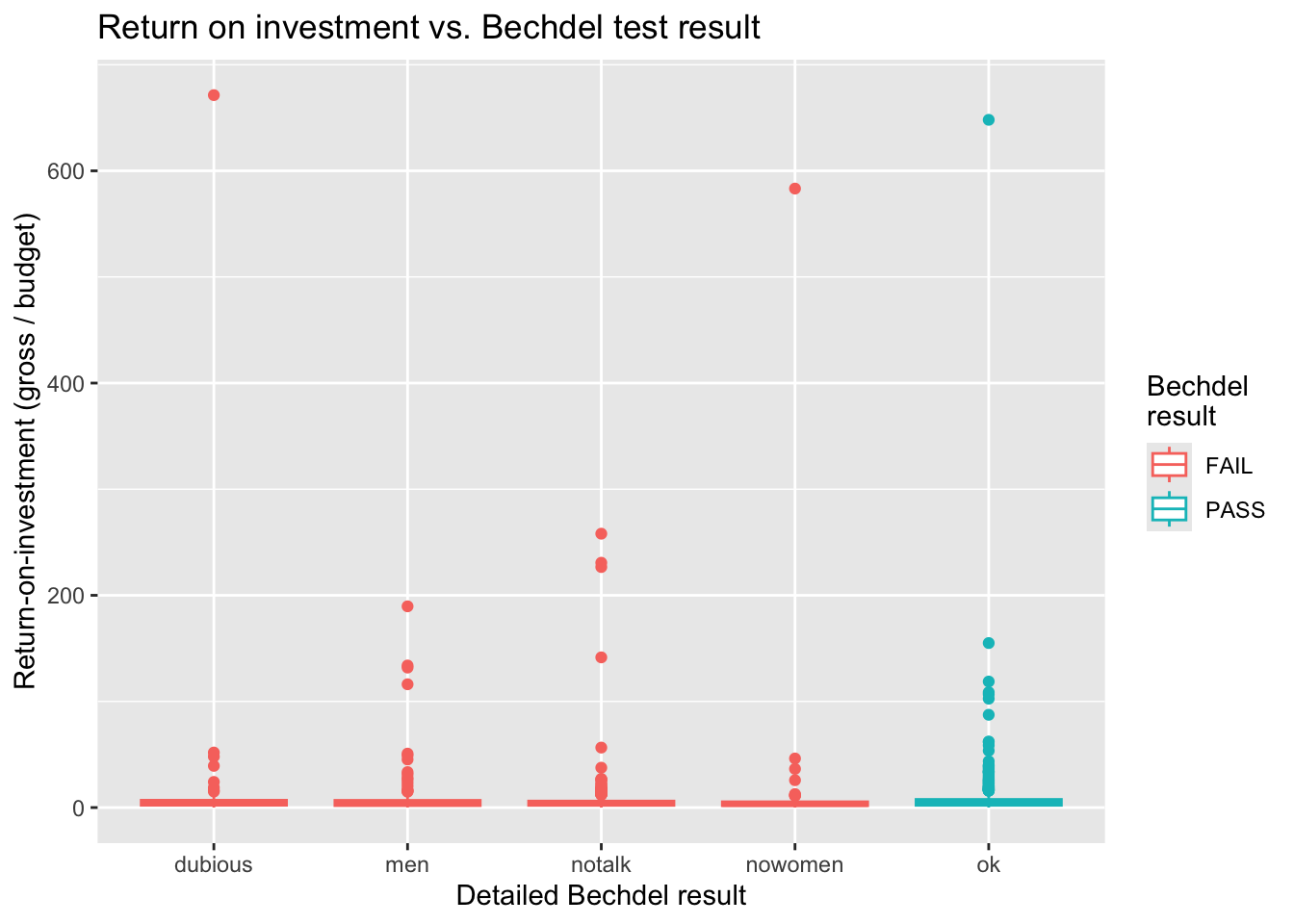

What are those movies with very high returns on investment?

bechdel |>
  filter(roi > 400) |>
  select(title, roi, budget_2013, gross_2013, year, clean_test)

# A tibble: 3 × 6
  title                     roi budget_2013 gross_2013  year clean_test
  <chr>                   <dbl>       <dbl>      <dbl> <dbl> <chr>     
1 Paranormal Activity      671.      505595  339424558  2007 dubious   
2 The Blair Witch Project  648.      839077  543776715  1999 ok        
3 El Mariachi              583.       11622    6778946  1992 nowomen

Step 2 - Demo

Expand on your plot from the previous step to zoom in on movies with roi < ___ to get a better view of how the medians across the categories compare.

ggplot(bechdel, aes(x = clean_test, y = roi, color = binary)) +
  geom_boxplot() +
  labs(
    title = "Return on investment vs. Bechdel test result",
    x = "Detailed Bechdel result",
    y = "Return-on-investment (gross / budget)",
    color = "Bechdel\nresult"
  ) +
  coord_cartesian(ylim = c(0, 16))

Warning: Removed 15 rows containing non-finite outside the scale range
(`stat_boxplot()`).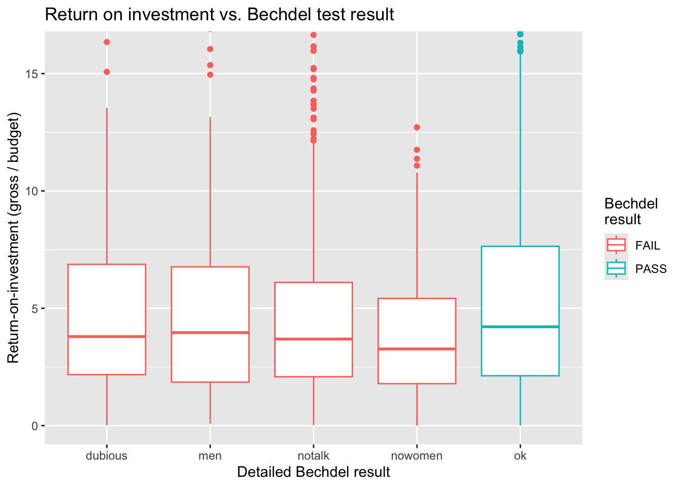

What does this plot say about return-on-investment on movies that pass the Bechdel test?

Render, commit, and push

Render your Quarto document.
Go to the Git pane and check the box next to each file listed, i.e., stage your changes. Commit your staged changes using a simple and informative message.
Click on push (the green arrow) to push your changes to your application exercise repo on GitHub.
Go to your repo on GitHub and confirm that you can see the updated files. Once your updated files are in your repo on GitHub, you’re good to go!