AE 05: Gerrymandering + data exploration II

Getting started

Packages

We’ll use the tidyverse package for this analysis.

library(tidyverse)
library(usdata)
library(ggbeeswarm)
library(ggthemes)
library(scales)

Data

The data are availale in the usdata package.

glimpse(gerrymander)

Rows: 435
Columns: 12
$ district   <chr> "AK-AL", "AL-01", "AL-02", "AL-03", "AL-04", "AL-05", "AL-0…
$ last_name  <chr> "Young", "Byrne", "Roby", "Rogers", "Aderholt", "Brooks", "…
$ first_name <chr> "Don", "Bradley", "Martha", "Mike D.", "Rob", "Mo", "Gary",…
$ party16    <chr> "R", "R", "R", "R", "R", "R", "R", "D", "R", "R", "R", "R",…
$ clinton16  <dbl> 37.6, 34.1, 33.0, 32.3, 17.4, 31.3, 26.1, 69.8, 30.2, 41.7,…
$ trump16    <dbl> 52.8, 63.5, 64.9, 65.3, 80.4, 64.7, 70.8, 28.6, 65.0, 52.4,…
$ dem16      <dbl> 0, 0, 0, 0, 0, 0, 0, 1, 0, 0, 0, 0, 1, 0, 1, 0, 0, 0, 1, 0,…
$ state      <chr> "AK", "AL", "AL", "AL", "AL", "AL", "AL", "AL", "AR", "AR",…
$ party18    <chr> "R", "R", "R", "R", "R", "R", "R", "D", "R", "R", "R", "R",…
$ dem18      <dbl> 0, 0, 0, 0, 0, 0, 0, 1, 0, 0, 0, 0, 1, 1, 1, 0, 0, 0, 1, 0,…
$ flip18     <dbl> 0, 0, 0, 0, 0, 0, 0, 0, 0, 0, 0, 0, 0, 1, 0, 0, 0, 0, 0, 0,…
$ gerry      <fct> mid, high, high, high, high, high, high, high, mid, mid, mi…

Congressional districts per state

Which state has the most congressional districts? How many congressional districts are there in this state?

gerrymander |>
  count(state, sort = TRUE)

# A tibble: 50 × 2
   state     n
   <chr> <int>
 1 CA       53
 2 TX       36
 3 FL       27
 4 NY       27
 5 IL       18
 6 PA       18
 7 OH       16
 8 GA       14
 9 MI       14
10 NC       13
# ℹ 40 more rows

California has the most, with 53 congressional districts.

Gerrymandering and flipping

Is a Congressional District more likely to be flipped to a Democratic seat if it has high prevalence of gerrymandering or low prevalence of gerrymandering? Support your answer with a visualization and summary statistics.

gerrymander |>
  mutate(flip18 = as_factor(flip18)) |>
  ggplot(aes(y = gerry, fill = flip18)) +
  geom_bar(position = "fill")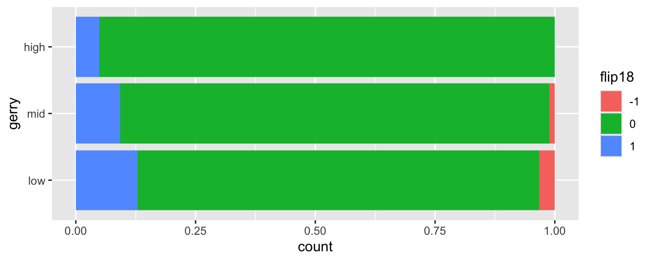

gerrymander |>
  count(gerry, dem18) |>
  group_by(gerry) |>
  mutate(p = n / sum(n))

# A tibble: 6 × 4
# Groups:   gerry [3]
  gerry dem18     n     p
  <fct> <dbl> <int> <dbl>
1 low       0    25 0.403
2 low       1    37 0.597
3 mid       0   131 0.485
4 mid       1   139 0.515
5 high      0    52 0.505
6 high      1    51 0.495

If a district is highly gerrymandered, it’s less likely to flip in general, no matter what the party is. As gerrymandering goes down (high → mid → low), both parties get more of a shot. 2018 was the first midterm election after the Republicans claimed the White House and Congress in 2016. Historically, such midterms favor the opposition party, so Democrats did more flipping across the board here. But the trend is that you get more flipping of all kinds in less gerrymandered districts.

Aesthetic mappings

Recreate the following visualization, and then improve it.

Recreate

ggplot(gerrymander, aes(x = gerry, y = clinton16, color = gerry)) +
  geom_beeswarm(color = "gray50", alpha = 0.5) +
  geom_boxplot(alpha = 0.5) +
  theme_minimal()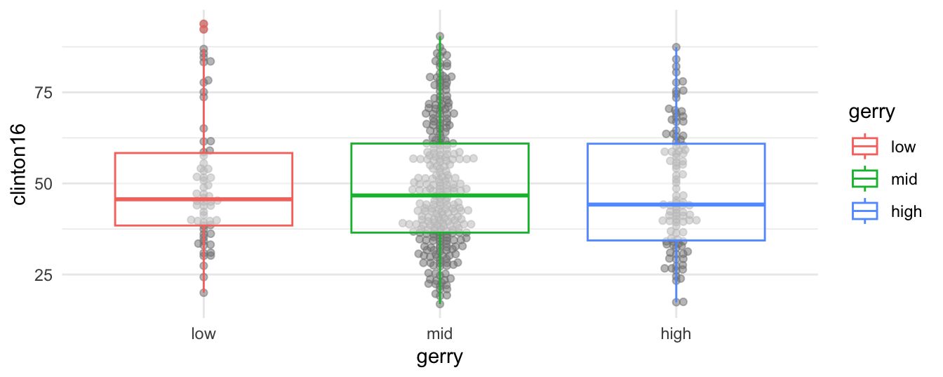

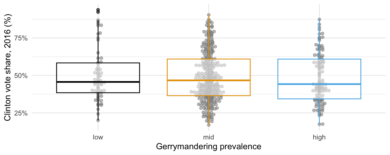
Improve

ggplot(gerrymander, aes(x = gerry, y = clinton16)) +
  geom_beeswarm(color = "gray50", alpha = 0.5) +
  geom_boxplot(
    aes(color = gerry),
    alpha = 0.5,
    show.legend = FALSE
  ) +
  scale_color_colorblind() +
  scale_y_continuous(labels = label_percent(scale = 1)) +
  theme_minimal() +
  labs(
    x = "Gerrymandering prevalence",
    y = "Clinton vote share, 2016 (%)",
  )