install.packages("palmerpenguins")Meet the toolkit
Lecture 1
Preliminaries
Reminders
- Complete Lab 0 ASAP;
- Don’t forget the
Getting to know yousurvey; - Accept your GitHub invitation pronto;
- Submit your SDAO letters and make testing center appointments now;
- Start lurking on Ed. Questions are being answered!
Updates
- There will be
eightseven homeworks. HW 1 appears next week; - Office hours are posted and begin today.
Questions?
How do we pronounce this?
STA 199
Last time
Spring break splits the class into two parts:
- Data science:
- convert data into knowledge;
- take a spreadsheet and compress it into pictures and a concise set of numerical summaries;
- try to teach a reader about the world or convince them of a claim;
- Statistical thinking:
- quantify our uncertainty about the results produced above;
- use this to make tricky decisions.
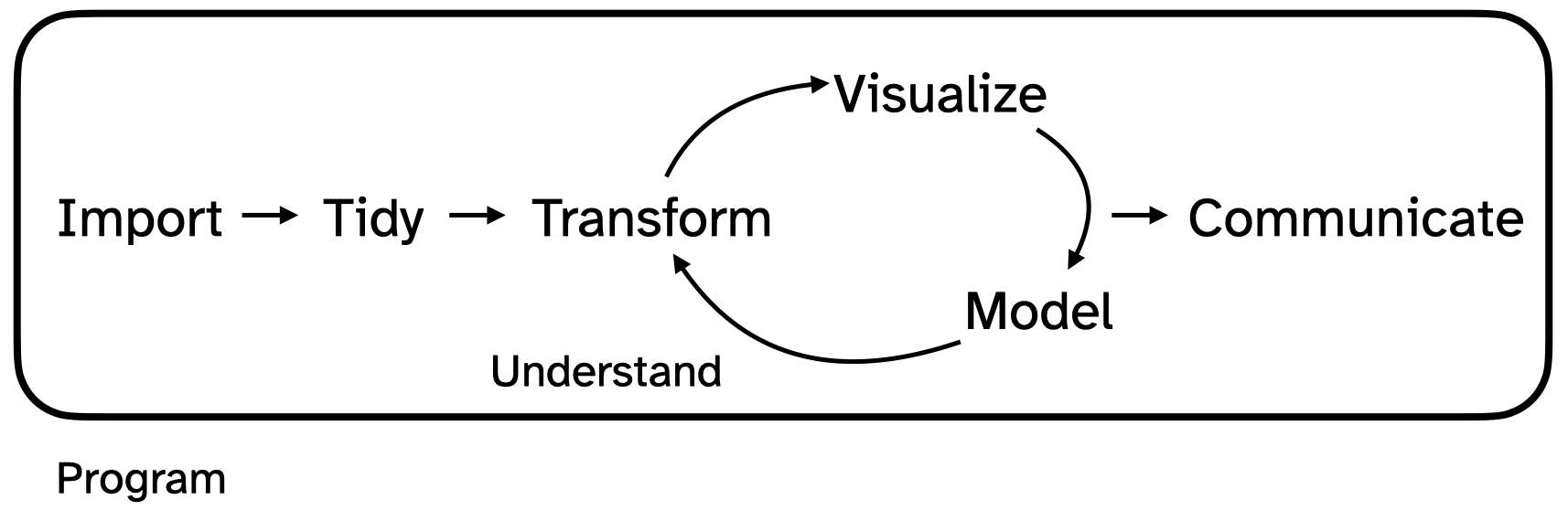
The data science life cycle
You will learn how to use a computer to actually do the following:
. . .
. . .
We emphasize technique (how do you make literally anything happen), but we also want you to develop good taste so that you can do these things well and convincingly.
Managing expectations
- Today is the first time all 300+ of us are attempting to access our containers simultaneously;
- I have yet to see this work the first time;
- After we get over the hump: smooth sailing;
- Until then: blood bath;
- Raise your hand if you need anything;
- If today is not your day, just sit back and watch.
Today and for forever
Please ask questions!
- Ask JZ: general interest questions about the presentation;
- Ask TA: technical questions about your particular computer.
Course toolkit
Course toolkit
Course operation
- Materials: sta199-s26.github.io
- Submission: Gradescope (in Canvas)
- Content Q&A: Ed Discussion (in Canvas)
- Grades: Gradebook (in Canvas)
Doing data science
- Computing:
- R
- RStudio
-
tidyverseand friends - Quarto
- Version control:
- Git
- GitHub
Toolkit: Computing
Learning goals
By the end of the course, you will be able to…
- gain insight from data
- gain insight from data, reproducibly
- gain insight from data, reproducibly, using modern programming tools and techniques
- gain insight from data, reproducibly and collaboratively, using modern programming tools and techniques
- gain insight from data, reproducibly (with literate programming and version control) and collaboratively, using modern programming tools and techniques
Two important concepts
. . .
Computational reproducibility:
- If you give me your code and your data and I hit “Run,” do I get the same numbers and the same pictures that you published in your article?
- If so…phew!
- If not…what the 🤬?
. . .
Scientific replication:
. . .
- Can new researchers conduct an independent analysis and reach the same substantive conclusions that you did?
- Just because your analysis is computationally reproducible does not mean that you have a robust result that generalizes.
. . .
Our tools will help you achieve the first, which is necessary (but not sufficient!) for the second.
Reproducibility checklist
What does it mean for a data analysis to be “reproducible”?
. . .
Short-term goals:
- Are the tables and figures reproducible from the code and data?
- Does the code actually do what you think it does?
- In addition to what was done, is it clear why it was done?
. . .
Long-term goals:
- Can the code be used for other data?
- Can you extend the code to do other things?
Toolkit for reproducibility
- Scriptability – Coding instead of point-and-click \(\rightarrow\) R
- Literate programming – code, written text, results all in one place instead of error-prone copy-paste \(\rightarrow\) Quarto
- Version control – Track changes with brief messages that describe those changes \(\rightarrow\) Git / GitHub
Collaboration
- Collaboration doesn’t just mean working with others. It also means collaborating with yourself across time;
- Too often, I have set something aside only to return to it several weeks (or even days!) later and ask “who did this and what were they thinking?”
- Our tools will make you an excellent collaborator with others, but they will also help you keep yourself organized.
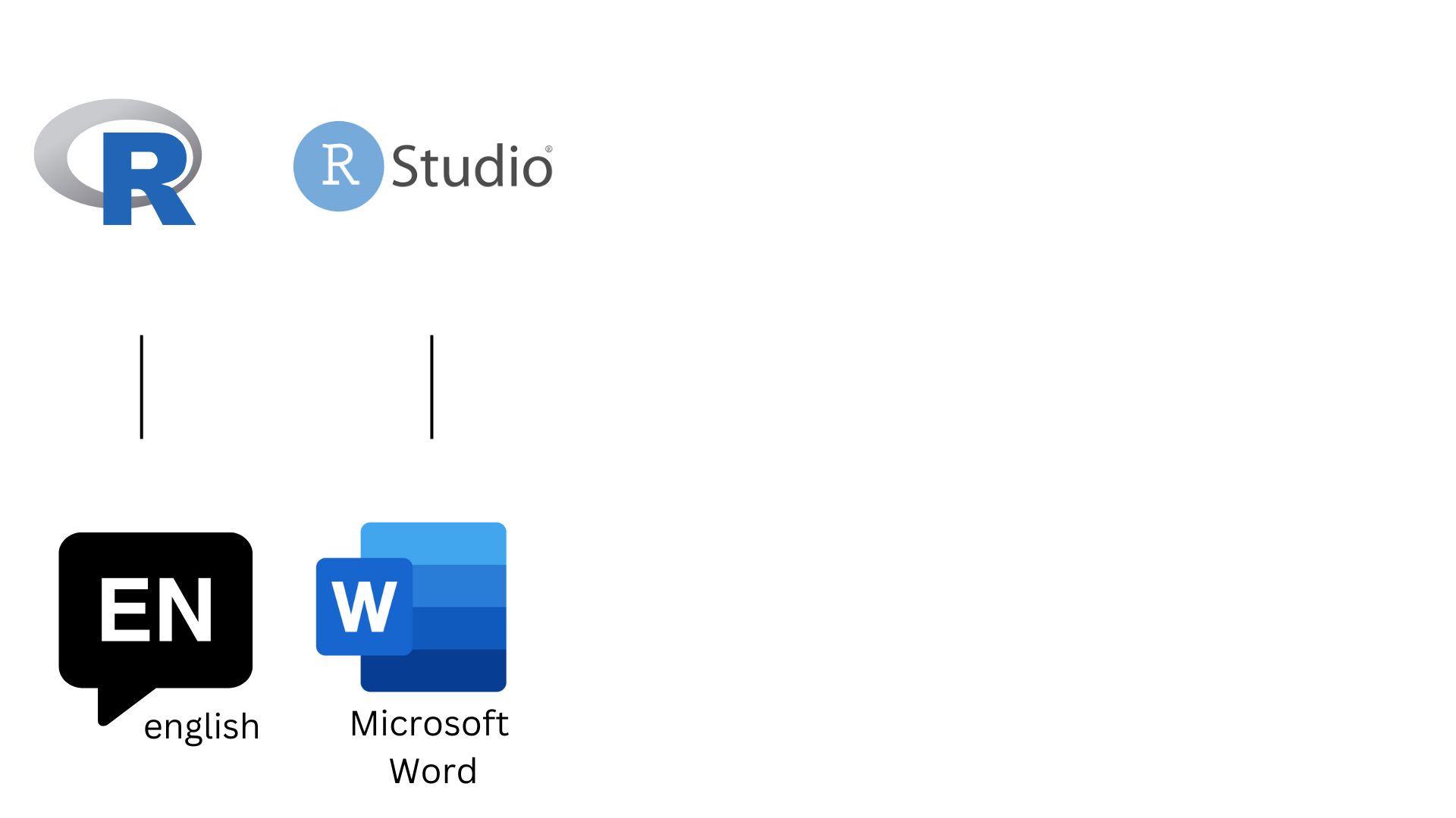
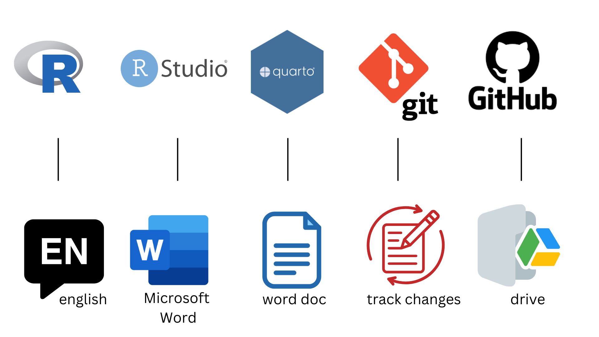
An Analogy to English
. . .

An Analogy to English
An Analogy to English
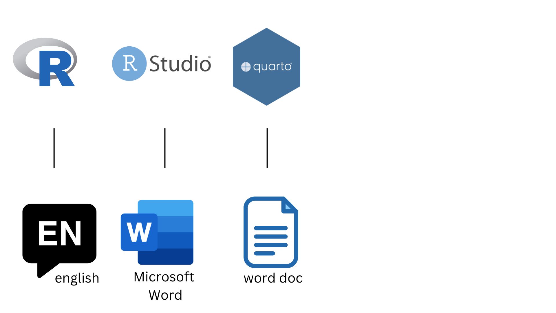
An Analogy to English
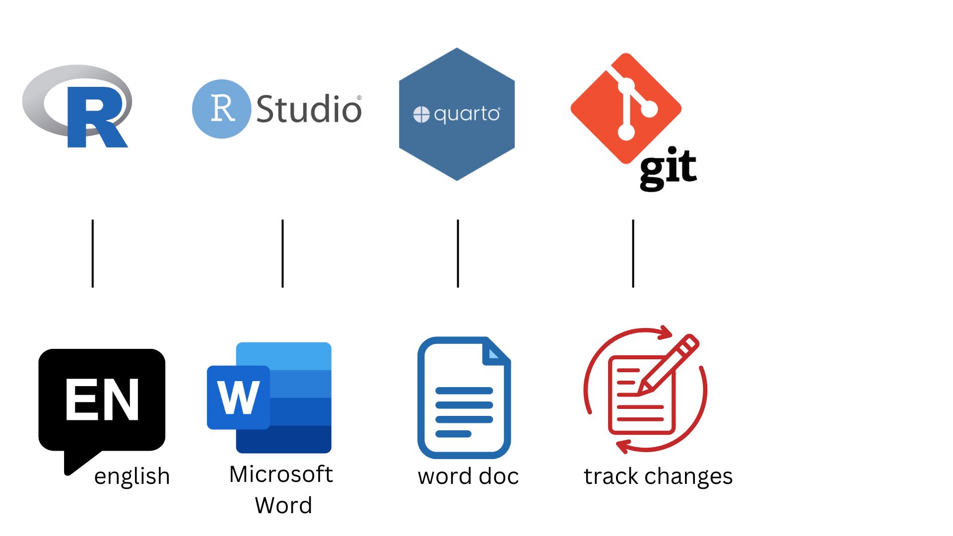
An Analogy to English
R and RStudio
R and RStudio
![]()
- R is an open-source statistical programming language
- R is also an environment for statistical computing and graphics
- It’s easily extensible with packages
![]()
- RStudio is a convenient interface for R called an IDE (integrated development environment), e.g. “I write R code in the RStudio IDE”
- RStudio is not a requirement for programming with R, but it’s very commonly used by R programmers and data scientists
R vs. RStudio
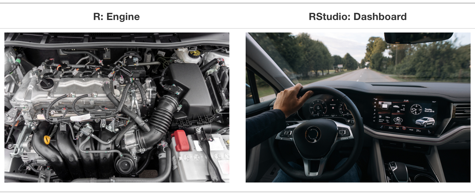
Source: Modern Dive.
R packages
Packages: Fundamental units of reproducible R code, including reusable R functions, the documentation that describes how to use them, and sample data1
As of 27 August 2025, there are 22,578 R packages available on CRAN (the Comprehensive R Archive Network)2
We’re going to work with a small (but important) subset of these!
1 Wickham and Bryan, R Packages.
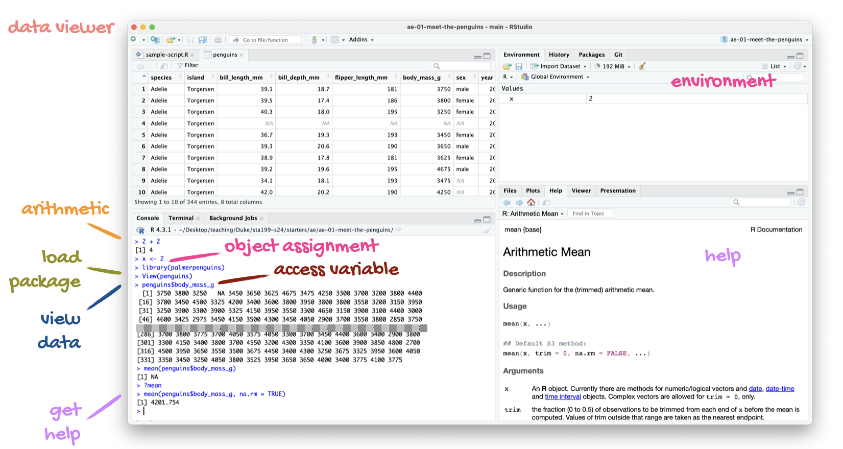
Tour: R + RStudio
Option 1:
Sit back and enjoy the show!
Option 2:
Go to your container and launch RStudio.
Tour recap: R + RStudio
A short list
(for now)
of R essentials
Packages
- Installed with
install.packages(), once per system:
Note
We already pre-installed many of the package you’ll need for this course, so you might go the whole semester without needing to run install.packages()!
. . .
- Loaded with
library(), once per session:
Attaching package: 'palmerpenguins'The following objects are masked from 'package:datasets':
penguins, penguins_rawData frames and variables
- Each row of a data frame is an observation
. . .
- Each column of a data frame is a variable
. . .
- Columns (variables) in data frames can be accessed with
$:
dataframe$variable_name
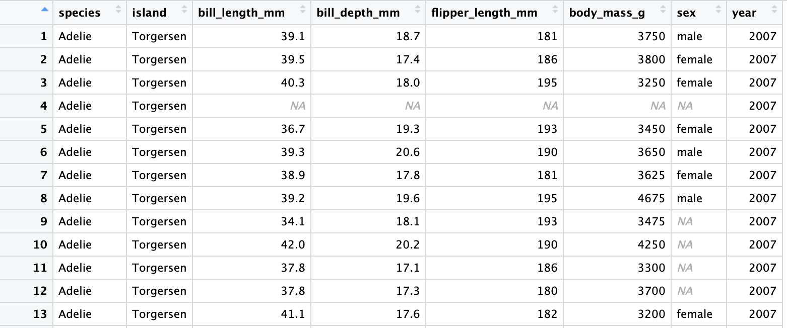
penguins data frame
penguins# A tibble: 344 × 8
species island bill_length_mm bill_depth_mm flipper_length_mm body_mass_g
<fct> <fct> <dbl> <dbl> <int> <int>
1 Adelie Torgersen 39.1 18.7 181 3750
2 Adelie Torgersen 39.5 17.4 186 3800
3 Adelie Torgersen 40.3 18 195 3250
4 Adelie Torgersen NA NA NA NA
5 Adelie Torgersen 36.7 19.3 193 3450
6 Adelie Torgersen 39.3 20.6 190 3650
7 Adelie Torgersen 38.9 17.8 181 3625
8 Adelie Torgersen 39.2 19.6 195 4675
9 Adelie Torgersen 34.1 18.1 193 3475
10 Adelie Torgersen 42 20.2 190 4250
# ℹ 334 more rows
# ℹ 2 more variables: sex <fct>, year <int>bill_length_mm
penguins$bill_length_mm [1] 39.1 39.5 40.3 NA 36.7 39.3 38.9 39.2 34.1 42.0 37.8 37.8 41.1 38.6 34.6
[16] 36.6 38.7 42.5 34.4 46.0 37.8 37.7 35.9 38.2 38.8 35.3 40.6 40.5 37.9 40.5
[31] 39.5 37.2 39.5 40.9 36.4 39.2 38.8 42.2 37.6 39.8 36.5 40.8 36.0 44.1 37.0
[46] 39.6 41.1 37.5 36.0 42.3 39.6 40.1 35.0 42.0 34.5 41.4 39.0 40.6 36.5 37.6
[61] 35.7 41.3 37.6 41.1 36.4 41.6 35.5 41.1 35.9 41.8 33.5 39.7 39.6 45.8 35.5
[76] 42.8 40.9 37.2 36.2 42.1 34.6 42.9 36.7 35.1 37.3 41.3 36.3 36.9 38.3 38.9
[91] 35.7 41.1 34.0 39.6 36.2 40.8 38.1 40.3 33.1 43.2 35.0 41.0 37.7 37.8 37.9
[106] 39.7 38.6 38.2 38.1 43.2 38.1 45.6 39.7 42.2 39.6 42.7 38.6 37.3 35.7 41.1
[121] 36.2 37.7 40.2 41.4 35.2 40.6 38.8 41.5 39.0 44.1 38.5 43.1 36.8 37.5 38.1
[136] 41.1 35.6 40.2 37.0 39.7 40.2 40.6 32.1 40.7 37.3 39.0 39.2 36.6 36.0 37.8
[151] 36.0 41.5 46.1 50.0 48.7 50.0 47.6 46.5 45.4 46.7 43.3 46.8 40.9 49.0 45.5
[166] 48.4 45.8 49.3 42.0 49.2 46.2 48.7 50.2 45.1 46.5 46.3 42.9 46.1 44.5 47.8
[181] 48.2 50.0 47.3 42.8 45.1 59.6 49.1 48.4 42.6 44.4 44.0 48.7 42.7 49.6 45.3
[196] 49.6 50.5 43.6 45.5 50.5 44.9 45.2 46.6 48.5 45.1 50.1 46.5 45.0 43.8 45.5
[211] 43.2 50.4 45.3 46.2 45.7 54.3 45.8 49.8 46.2 49.5 43.5 50.7 47.7 46.4 48.2
[226] 46.5 46.4 48.6 47.5 51.1 45.2 45.2 49.1 52.5 47.4 50.0 44.9 50.8 43.4 51.3
[241] 47.5 52.1 47.5 52.2 45.5 49.5 44.5 50.8 49.4 46.9 48.4 51.1 48.5 55.9 47.2
[256] 49.1 47.3 46.8 41.7 53.4 43.3 48.1 50.5 49.8 43.5 51.5 46.2 55.1 44.5 48.8
[271] 47.2 NA 46.8 50.4 45.2 49.9 46.5 50.0 51.3 45.4 52.7 45.2 46.1 51.3 46.0
[286] 51.3 46.6 51.7 47.0 52.0 45.9 50.5 50.3 58.0 46.4 49.2 42.4 48.5 43.2 50.6
[301] 46.7 52.0 50.5 49.5 46.4 52.8 40.9 54.2 42.5 51.0 49.7 47.5 47.6 52.0 46.9
[316] 53.5 49.0 46.2 50.9 45.5 50.9 50.8 50.1 49.0 51.5 49.8 48.1 51.4 45.7 50.7
[331] 42.5 52.2 45.2 49.3 50.2 45.6 51.9 46.8 45.7 55.8 43.5 49.6 50.8 50.2Why did the error occur?
flipper_length_mmError: object 'flipper_length_mm' not foundflipper_length_mm
This can be fixed by using penguins$flipper_length_mm.
penguins$flipper_length_mm [1] 181 186 195 NA 193 190 181 195 193 190 186 180 182 191 198 185 195 197
[19] 184 194 174 180 189 185 180 187 183 187 172 180 178 178 188 184 195 196
[37] 190 180 181 184 182 195 186 196 185 190 182 179 190 191 186 188 190 200
[55] 187 191 186 193 181 194 185 195 185 192 184 192 195 188 190 198 190 190
[73] 196 197 190 195 191 184 187 195 189 196 187 193 191 194 190 189 189 190
[91] 202 205 185 186 187 208 190 196 178 192 192 203 183 190 193 184 199 190
[109] 181 197 198 191 193 197 191 196 188 199 189 189 187 198 176 202 186 199
[127] 191 195 191 210 190 197 193 199 187 190 191 200 185 193 193 187 188 190
[145] 192 185 190 184 195 193 187 201 211 230 210 218 215 210 211 219 209 215
[163] 214 216 214 213 210 217 210 221 209 222 218 215 213 215 215 215 216 215
[181] 210 220 222 209 207 230 220 220 213 219 208 208 208 225 210 216 222 217
[199] 210 225 213 215 210 220 210 225 217 220 208 220 208 224 208 221 214 231
[217] 219 230 214 229 220 223 216 221 221 217 216 230 209 220 215 223 212 221
[235] 212 224 212 228 218 218 212 230 218 228 212 224 214 226 216 222 203 225
[253] 219 228 215 228 216 215 210 219 208 209 216 229 213 230 217 230 217 222
[271] 214 NA 215 222 212 213 192 196 193 188 197 198 178 197 195 198 193 194
[289] 185 201 190 201 197 181 190 195 181 191 187 193 195 197 200 200 191 205
[307] 187 201 187 203 195 199 195 210 192 205 210 187 196 196 196 201 190 212
[325] 187 198 199 201 193 203 187 197 191 203 202 194 206 189 195 207 202 193
[343] 210 198function(argument)
Functions are (most often) verbs, followed by what they will be applied to in parentheses:
do_this(to_this)
do_that(to_this, to_that, with_those)
mean()
Let’s compute the average of a set of numbers:
x <- c(1, 2, 3, 4, 5, 6, 7, 8, 9)
x
[1] 1 2 3 4 5 6 7 8 9. . .
mean(x)[1] 5mean()
mean(penguins$flipper_length_mm)[1] NA. . .
Wut?
. . .
head(penguins$flipper_length_mm)[1] 181 186 195 NA 193 190. . .
There’s a missing value (NA stands for “not available”).
. . .
mean(penguins$flipper_length_mm, na.rm = TRUE)[1] 200.9152Help
Object documentation can be accessed with ?
?meanSummary of R essentials
- Functions are (most often) verbs, followed by what they will be applied to in parentheses:
do_this(to_this)
do_that(to_this, to_that, with_those)- Packages are installed with the
install.packages()function and loaded with thelibraryfunction, once per session:
install.packages("package_name")
library(package_name)
Your containers come “fully loaded,” so you may not have to install any new packages.
Summary of R essentials (continued)
Data frames: like the spreadsheets of R
- Each row of a data frame is an observation
- Each column of a data frame is a variable
Summary of R essentials (continued)
- Use the question mark
?to get help with objects (like data frames and functions):
?function_name- Use the dollar sign
$to access columns
dataframe$column
Note
Generally, you need to use the $ to tell R where to find that column.
Summary of R essentials (continued)
- Use the arrow
<-or equals sign=to save objects
x = some_thing
y <- some_other_thing
Note
Check your environment pane for the saved object!
Summary of R essentials (continued)
- Read your error messages!
- These are essential for figuring out where your code is going wrong.
Note
If you have trouble understanding what a message is saying, there is a high chance someone has explained the message online.
Packages, an analogy
If data analysis was cooking…
Installing a package would be like buying ingredients from the store
Loading a package would be like getting the ingredients out of your pantry and setting them on your counter top to be used
tidyverse
aka the package you’ll hear about the most…
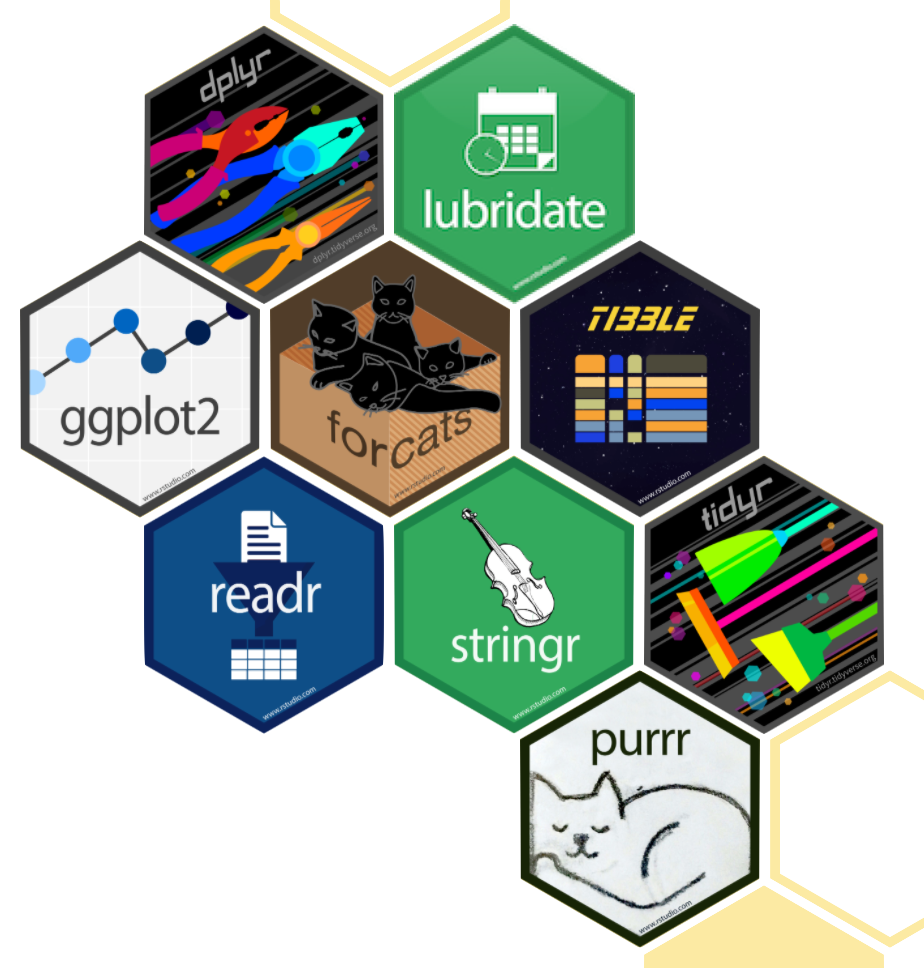
- The tidyverse is an opinionated collection of R packages designed for data science
- All packages share an underlying philosophy and a common grammar
Toolkit: Version control and collaboration
Git and GitHub
![]()
- Git is a version control system – like “Track Changes” features from Microsoft Word, on steroids
- It’s not the only version control system, but it’s a very popular one
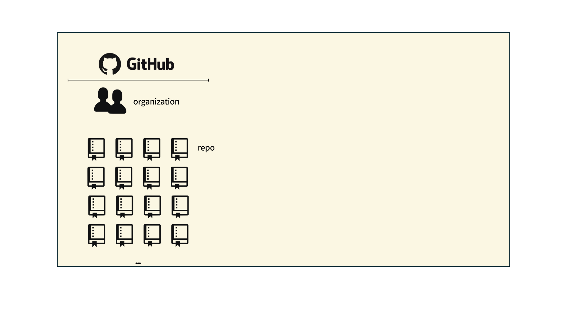
![]()
GitHub is the home for your Git-based projects on the internet – like DropBox but much, much better
We will use GitHub as a platform for web hosting and collaboration (and as our course management system!)
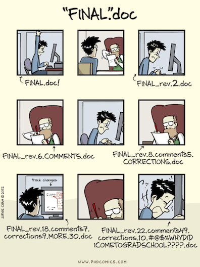
Versioning - done badly
Versioning - done better
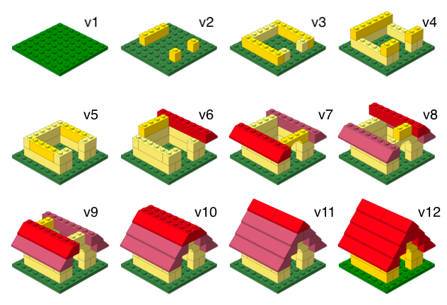
Versioning - done even better
with human readable messages

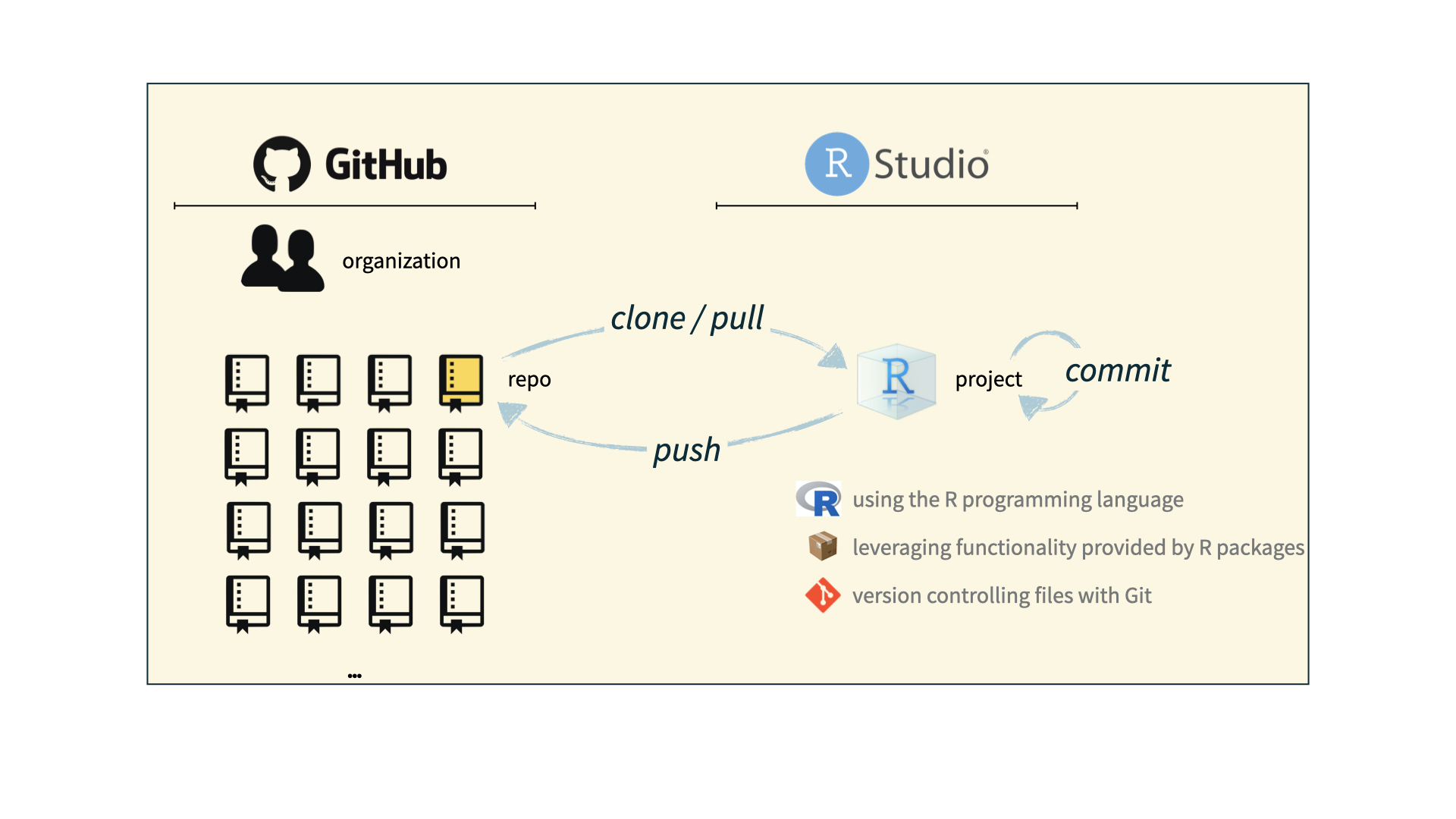
How will we use Git and GitHub?
How will we use Git and GitHub?
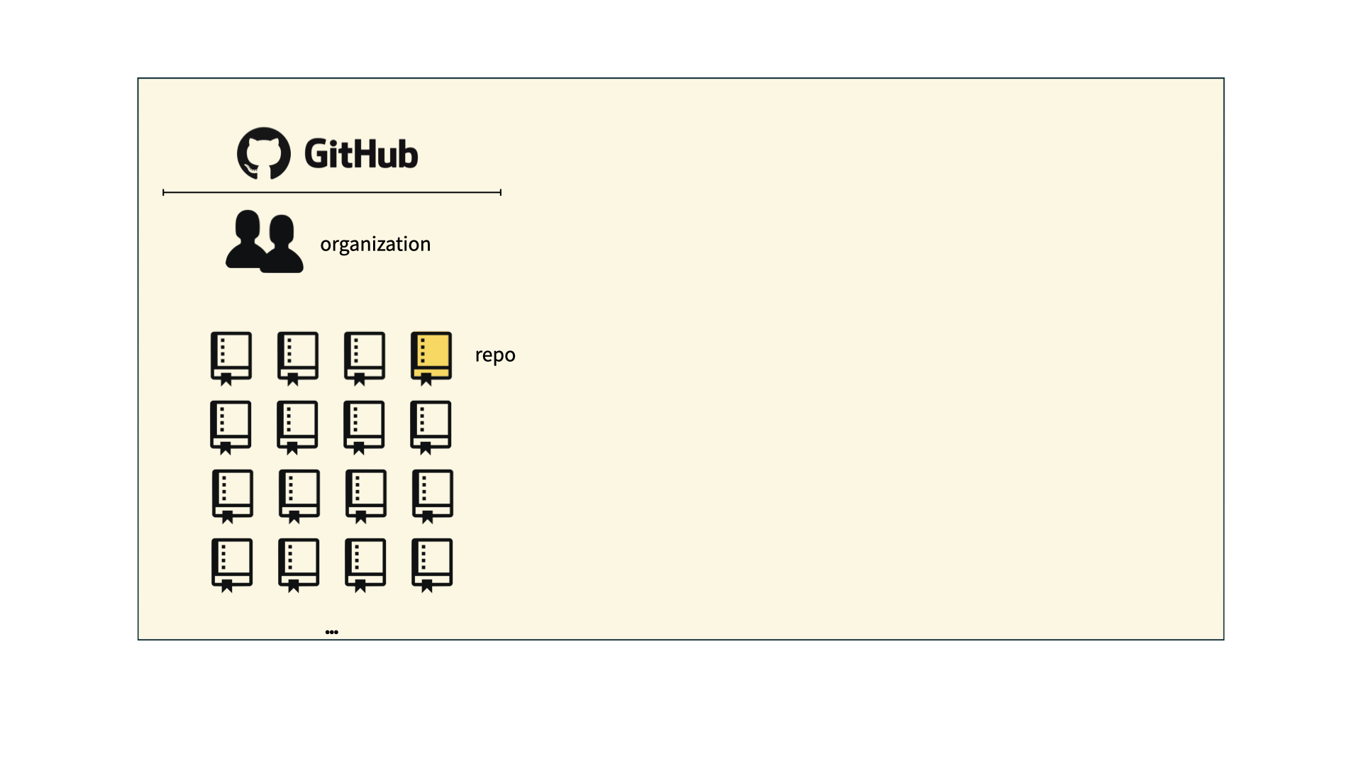
How will we use Git and GitHub?
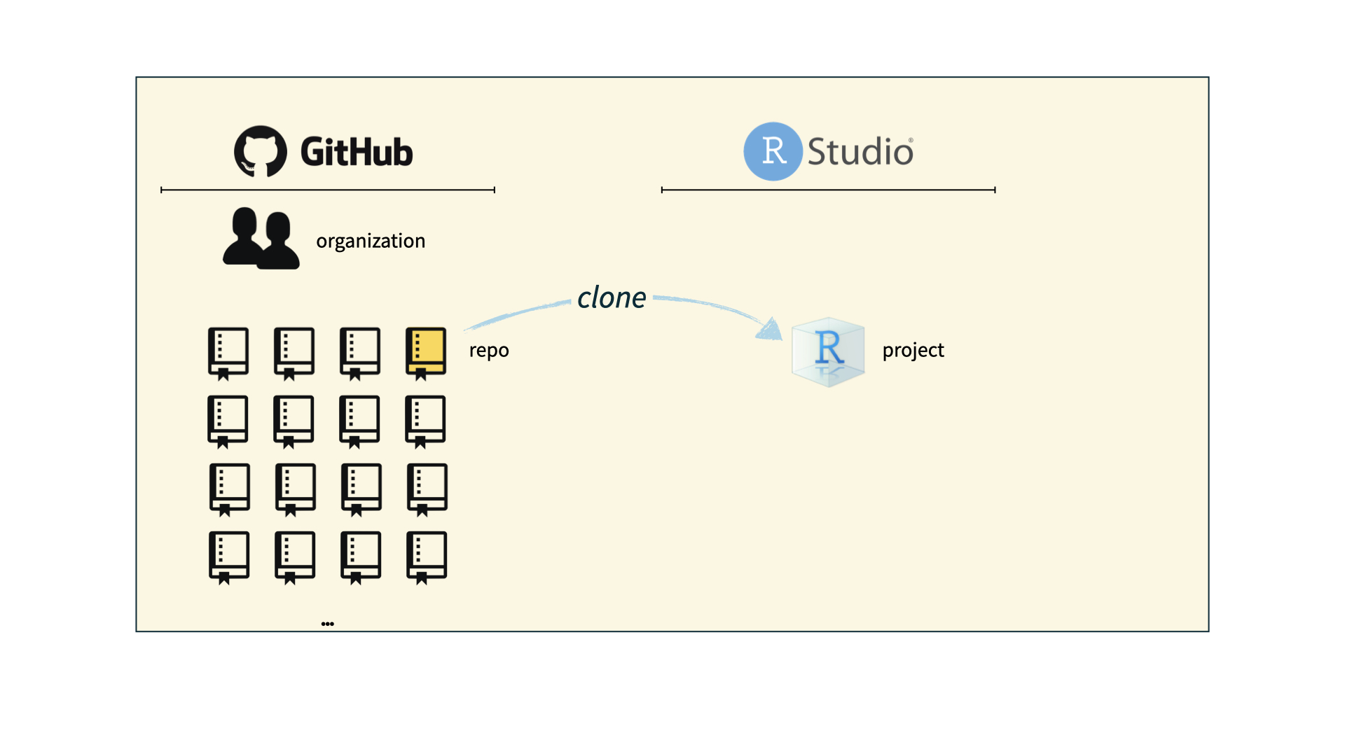
How will we use Git and GitHub?
Git and GitHub tips
- There are millions of git commands – ok, that’s an exaggeration, but there are a lot of them – and very few people know them all. 99% of the time you will use git to add, commit, push, and pull.
- We will be doing Git things and interfacing with GitHub through RStudio, but if you google for help you might come across methods for doing these things in the command line – skip that and move on to the next resource unless you feel comfortable trying it out.
- There is a great resource for working with git and R: happygitwithr.com. Some of the content in there is beyond the scope of this course, but it’s a good place to look for help.
Tour: Git + GitHub
Option 1:
Sit back and enjoy the show!
Note
You’ll need to stick to this option if you haven’t yet accepted your GitHub invite and don’t have a repo created for you.
Option 2:
Go to the course GitHub organization and clone ae-YOUR-GITHUB-NAME repo to your container.
Tour recap: Git + GitHub
Find your application repo, that will always be named using the naming convention
assignment_title-YOUR-GITHUB-NAME, e.g.,ae-johnczitoorlab-1-johnczito.Click on the green “Code” button, make sure SSH is selected, copy the repo URL
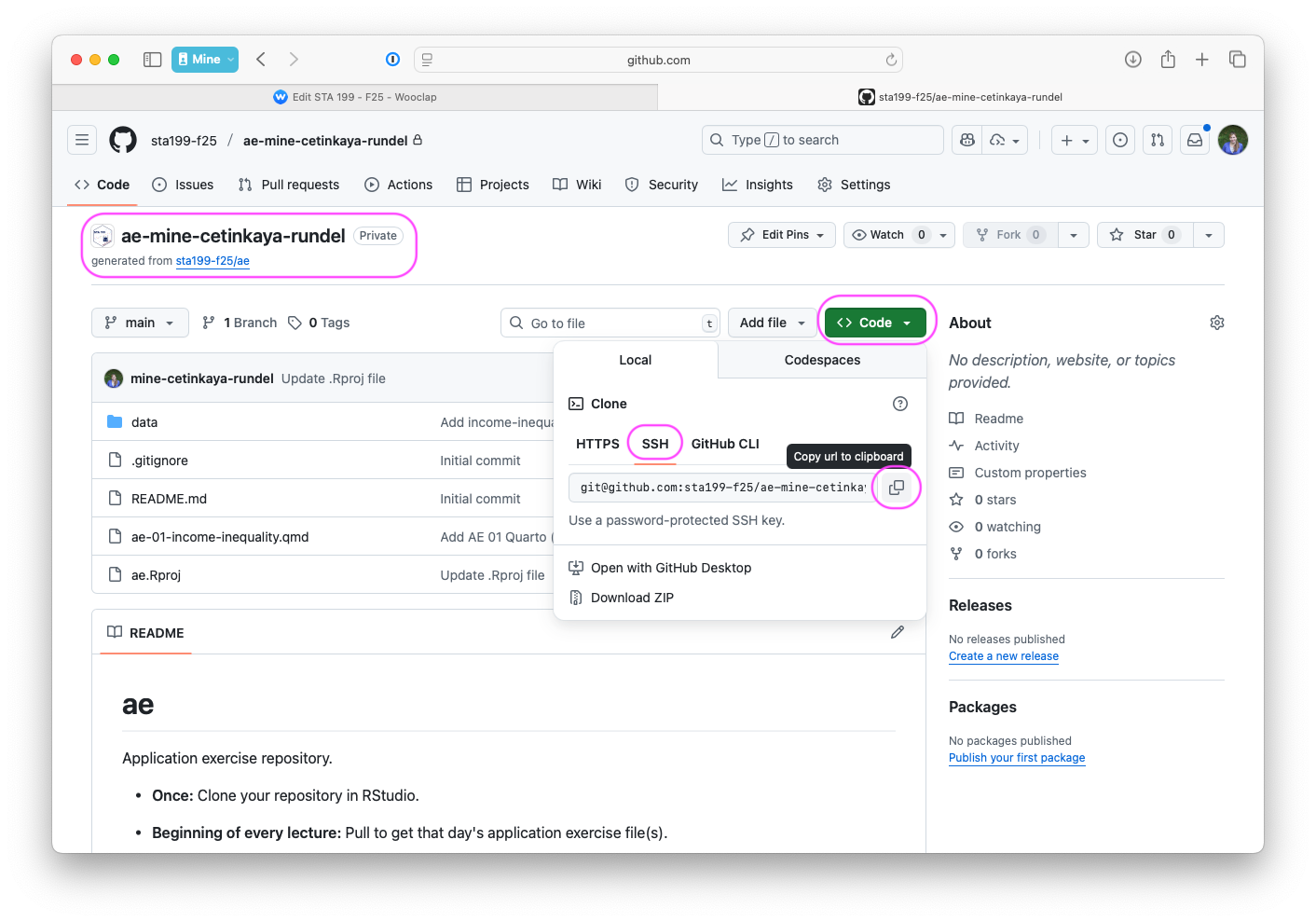
In RStudio, File > New Project > From Version Control > Git
Paste repo URL copied in previous step, then click tab to auto-fill the project name, then click Create Project
If you haven’t done Lab 0, for one time only, type
yesin the pop-up dialogue
What could have gone wrong?
Never received GitHub invite \(\rightarrow\) Fill out “Getting to know you survey
Never accepted GitHub invite \(\rightarrow\) Look for it in your email and accept it
Cloning repo fails \(\rightarrow\) Review/redo Lab 0 steps for setting up SSH key
Still no luck? Stay after class today or come by my office hours tomorrow or post on Ed for help
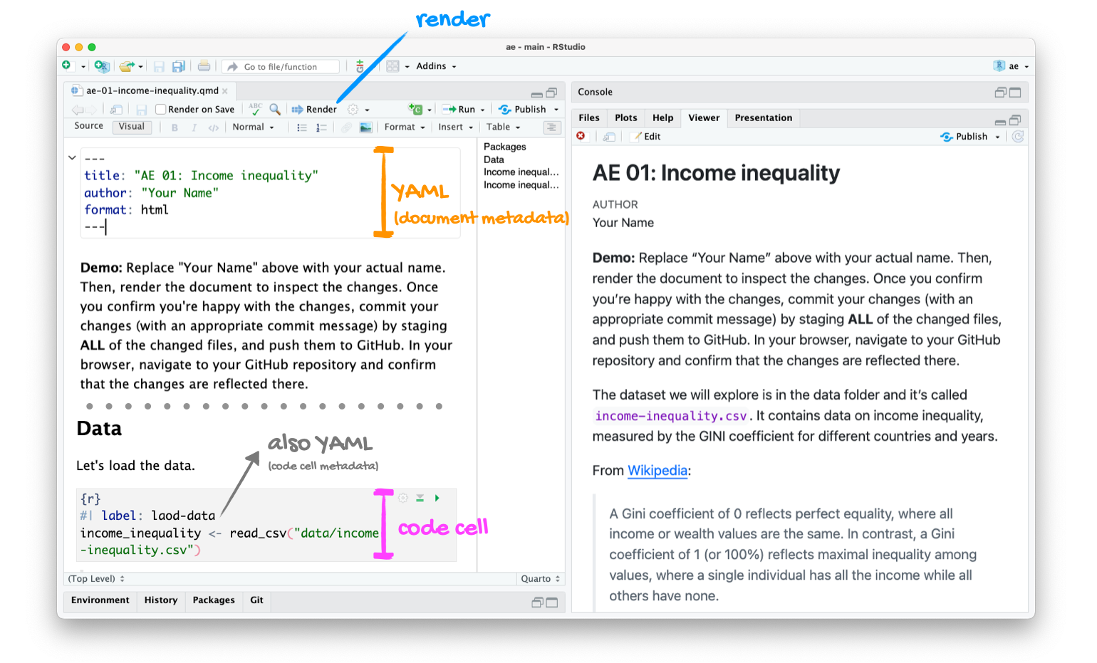
Quarto
Quarto
- Fully reproducible reports – each time you render the analysis is run from the beginning;
- Code goes in cells (between the three back ticks);
- Written English goes outside cells, the same way you would write in Google Docs or MS Word.
Tour: Quarto
Option 1:
Sit back and enjoy the show!
Note
If you chose (or had to choose) this option for the previous tour, or if you couldn’t clone your repo for any reason, you’ll need to stick to this option.
Option 2:
Go to RStudio and open the document ae-01-income-inequality.qmd.
Tour: Quarto (and more Git + GitHub)
Tour recap: Quarto
Tour recap: Git + GitHub
Once we made changes to our Quarto document, we
went to the Git pane in RStudio
staged our changes by clicking the checkboxes next to the relevant files
committed our changes with an informative commit message
pulled from GitHub to make sure we had the latest version of our repo
pushed our changes to our application exercise repos
confirmed on GitHub that we could see our changes pushed from RStudio
How will we use Quarto?
- Every application exercise, lab, project, etc. is an Quarto document
- You’ll always have a template Quarto document to start with
- The amount of scaffolding in the template will decrease over the semester