Joining data
Lecture 7
While you wait…
Prepare for today’s application exercise: ae-07-taxes-join
Go to your
aeproject in RStudio.Make sure all of your changes up to this point are committed and pushed, i.e., there’s nothing left in your Git pane.
Click Pull to get today’s application exercise file: ae-07-taxes-join.qmd.
Wait till the you’re prompted to work on the application exercise during class before editing the file.
Support your classmates this weekend!

- Paige Auditorium;
- Friday and Saturday @ 7pm;
- STAWANANA students in…
- Duke Chinese Dance
- Temptasians
- Defining Movement
- Club Taekwondo
- (what else?)
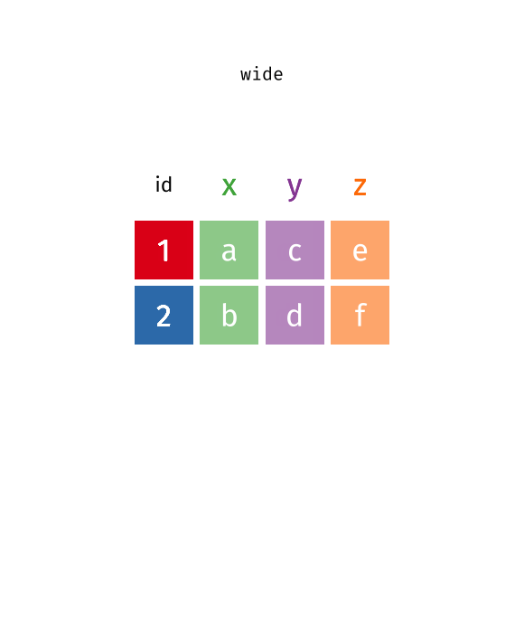
Recap: pivoting
Recoding data
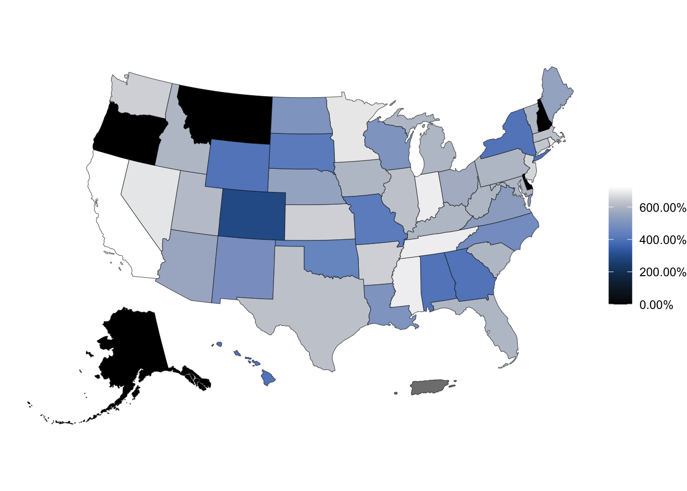
What’s going on in this plot?
Can you guess the variable plotted here?
Sales taxes in US states
sales_taxes# A tibble: 51 × 7
state state_tax_rate state_tax_rank avg_local_tax_rate max_local
<chr> <dbl> <dbl> <dbl> <dbl>
1 Alabama 4 40 5.44 11
2 Alaska 0 46 1.82 7.85
3 Arizona 5.6 28 2.92 5.3
4 Arkansas 6.5 9 2.98 6.12
5 California 7.25 1 1.73 5.25
6 Colorado 2.9 45 4.96 8.3
7 Connecticut 6.35 12 0 0
8 Delaware 0 46 0 0
9 Florida 6 17 1.02 2
10 Georgia 4 40 3.44 5
# ℹ 41 more rows
# ℹ 2 more variables: combined_tax_rate <dbl>, combined_rank <dbl>Sales tax in swing states
Suppose you’re tasked with the following:
Compare the average state sales tax rates of swing states (Arizona, Georgia, Michigan, Nevada, North Carolina, Pennsylvania, and Wisconsin) vs. non-swing states.
How would you approach this task?
. . .
- Create a new variable called
swing_statewith levels"Swing"and"Non-swing" - Group by
swing_state - Summarize to find the mean sales tax in each type of state
ae-07-taxes-join
Go to your ae project in RStudio.
If you haven’t yet done so, make sure all of your changes up to this point are committed and pushed, i.e., there’s nothing left in your Git pane.
If you haven’t yet done so, click Pull to get today’s application exercise file: ae-07-taxes-join.qmd.
Work through the application exercise in class, and render, commit, and push your edits by the end of class.
mutate() with if_else()
Create a new variable called swing_state with levels "Swing" and "Non-swing".
list_of_swing_states <- c("Arizona", "Georgia", "Michigan", "Nevada",
                          "North Carolina", "Pennsylvania", "Wisconsin")

sales_taxes <- sales_taxes |>
  mutate(
    swing_state = if_else(state %in% list_of_swing_states,
                          "Swing",
                          "Non-swing")) |>
  relocate(swing_state)

sales_taxes
# A tibble: 51 × 8
swing_state state state_tax_rate state_tax_rank avg_local_tax_rate max_local
<chr> <chr> <dbl> <dbl> <dbl> <dbl>
1 Non-swing Alaba… 4 40 5.44 11
2 Non-swing Alaska 0 46 1.82 7.85
3 Swing Arizo… 5.6 28 2.92 5.3
4 Non-swing Arkan… 6.5 9 2.98 6.12
5 Non-swing Calif… 7.25 1 1.73 5.25
6 Non-swing Color… 2.9 45 4.96 8.3
7 Non-swing Conne… 6.35 12 0 0
8 Non-swing Delaw… 0 46 0 0
9 Non-swing Flori… 6 17 1.02 2
10 Swing Georg… 4 40 3.44 5
# ℹ 41 more rows
# ℹ 2 more variables: combined_tax_rate <dbl>, combined_rank <dbl>Recap: if_else()
if_else(
  x == y,
  "x is equal to y",
  "x is not equal to y"
)- 1
- Condition
- 2
-
Value if condition is
TRUE - 3
-
Value if condition is
FALSE
Participate 📱💻
Fill in the blank to compare the average state sales tax rates of swing states vs. non-swing states.
sales_taxes |>
  __BLANK__ |>
summarize(mean_state_tax = mean(state_tax_rate))arrange(swing_state)filter(swing_state == "Swing")group_by(swing_state)group_by(list_of_swing_states)
Sales tax in swing states
Compare the average state sales tax rates of swing states vs. non-swing states.
sales_taxes |>
  group_by(swing_state) |>
  summarize(mean_state_tax = mean(state_tax_rate))
# A tibble: 2 × 2
swing_state mean_state_tax
<chr> <dbl>
1 Non-swing 5.05
2 Swing 5.46Sales tax in coastal states
Suppose you’re tasked with the following:
Compare the average state sales tax rates of states on the Pacific Coast, states on the Atlantic Coast, and the rest of the states.
How would you approach this task?
. . .
- Create a new variable called
coastwith levels"Pacific","Atlantic", and"Neither" - Group by
coast - Summarize to find the mean sales tax in each type of state
mutate() with case_when()
Create a new variable called coast with levels "Pacific", "Atlantic", and "Neither".
pacific_coast <- c("Alaska", "Washington", "Oregon", "California", "Hawaii")

atlantic_coast <- c(
  "Connecticut", "Delaware", "Georgia", "Florida", "Maine", "Maryland",
  "Massachusetts", "New Hampshire", "New Jersey", "New York",
  "North Carolina", "Rhode Island", "South Carolina", "Virginia"
)

sales_taxes <- sales_taxes |>
  mutate(
    coast = case_when(
      state %in% pacific_coast ~ "Pacific",
      state %in% atlantic_coast ~ "Atlantic",
      .default = "Neither"
    )
  ) |>
  relocate(coast)

sales_taxes
# A tibble: 51 × 9
coast swing_state state state_tax_rate state_tax_rank avg_local_tax_rate
<chr> <chr> <chr> <dbl> <dbl> <dbl>
1 Neither Non-swing Alabama 4 40 5.44
2 Pacific Non-swing Alaska 0 46 1.82
3 Neither Swing Arizona 5.6 28 2.92
4 Neither Non-swing Arkans… 6.5 9 2.98
5 Pacific Non-swing Califo… 7.25 1 1.73
6 Neither Non-swing Colora… 2.9 45 4.96
7 Atlantic Non-swing Connec… 6.35 12 0
8 Atlantic Non-swing Delawa… 0 46 0
9 Atlantic Non-swing Florida 6 17 1.02
10 Atlantic Swing Georgia 4 40 3.44
# ℹ 41 more rows
# ℹ 3 more variables: max_local <dbl>, combined_tax_rate <dbl>,
# combined_rank <dbl>Recap: case_when()
case_when(
  x > y  ~ "x is greater than y",
  x < y  ~ "x is less than y",
  .default = "x is equal to y"
)- 1
-
Value if first condition is
TRUE - 2
-
Value if second condition is
TRUE - 3
-
Value if neither condition is
TRUE, i.e., default value
Sales tax in coastal states
Compare the average state sales tax rates of states on the Pacific Coast, states on the Atlantic Coast, and the rest of the states.
sales_taxes |>
  group_by(coast) |>
  summarize(mean_state_tax = mean(state_tax_rate))
# A tibble: 3 × 2
coast mean_state_tax
<chr> <dbl>
1 Atlantic 4.84
2 Neither 5.46
3 Pacific 3.55Sales tax in US regions
Suppose you’re tasked with the following:
Compare the average state sales tax rates of states in various regions (Midwest - 12 states, Northeast - 9 states, South - 16 states, West - 13 states).
How would you approach this task?
. . .
- Create a new variable called
regionwith levels"Midwest","Northeast","South", and"West". - Group by
region - Summarize to find the mean sales tax in each type of state
mutate() with case_when()
Who feels like filling in the blanks lists of states in each region? Who feels like it’s simply too tedious to write out names of all states?
list_of_midwest_states <- c(___)
list_of_northeast_states <- c(___)
list_of_south_states <- c(___)
list_of_west_states <- c(___)

sales_taxes <- sales_taxes |>
  mutate(
    coast = case_when(
      state %in% list_of_west_states ~ "Midwest",
      state %in% list_of_northeast_states ~ "Northeast",
      state %in% list_of_south_states ~ "South",
      state %in% list_of_west_states ~ "West"
    )
  )
Joining data
Why join?
Suppose we want to answer questions like:
Is there a relationship between
- number of QS courses taken
- having scored a 4 or 5 on the AP stats exam
- motivation for taking course
- …
and performance in this course?”
. . .
Each of these would require joining class performance data with an outside data source so we can have all relevant information (columns) in a single data frame.
Why join?
Suppose we want to answer questions like:
Compare the average state sales tax rates of states in various regions (Midwest - 12 states, Northeast - 9 states, South - 16 states, West - 13 states).
. . .
This can also be solved with joining region information with the state-level sales tax data.
Setup
For the next few slides…
left_join()
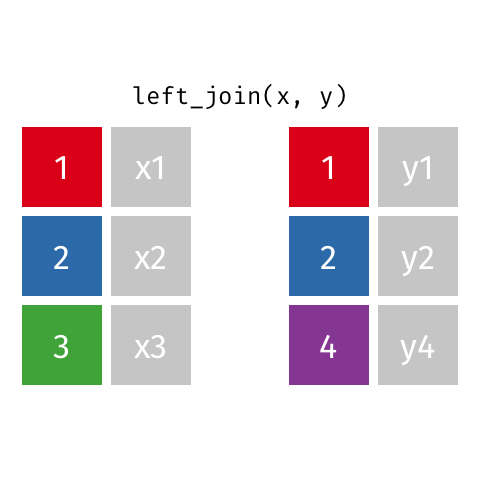
left_join(x, y)Joining with `by = join_by(id)`# A tibble: 3 × 3
id value_x value_y
<dbl> <chr> <chr>
1 1 x1 y1
2 2 x2 y2
3 3 x3 <NA> right_join()

right_join(x, y)Joining with `by = join_by(id)`# A tibble: 3 × 3
id value_x value_y
<dbl> <chr> <chr>
1 1 x1 y1
2 2 x2 y2
3 4 <NA> y4 full_join()
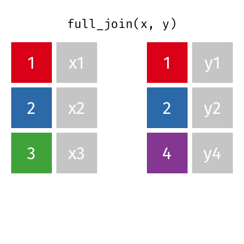
full_join(x, y)Joining with `by = join_by(id)`# A tibble: 4 × 3
id value_x value_y
<dbl> <chr> <chr>
1 1 x1 y1
2 2 x2 y2
3 3 x3 <NA>
4 4 <NA> y4 inner_join()
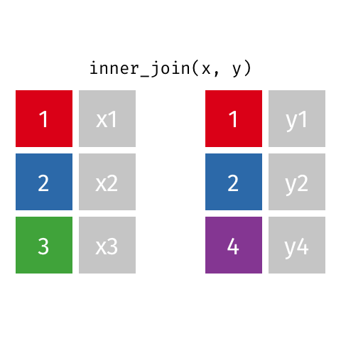
inner_join(x, y)Joining with `by = join_by(id)`# A tibble: 2 × 3
id value_x value_y
<dbl> <chr> <chr>
1 1 x1 y1
2 2 x2 y2 semi_join()

semi_join(x, y)Joining with `by = join_by(id)`# A tibble: 2 × 2
id value_x
<dbl> <chr>
1 1 x1
2 2 x2 anti_join()

anti_join(x, y)Joining with `by = join_by(id)`# A tibble: 1 × 2
id value_x
<dbl> <chr>
1 3 x3 Summary
