Logistic regression

Lecture 19

Author

Affiliation

Katie Solarz

Duke University
STA 199 Spring 2026

Published

March 30, 2026

While you wait: Participate 📱💻

What is the difference between the additive vs. interaction linear model when you run a regression model with one numeric and one categorical predictor?

This is a trick question - both models require only numeric predictors.
Both give you different lines for each group, but the additive model requires the lines be parallel.
Both give you different lines for each group, but the interaction model requires the lines be parallel.
Where is John Zito and what have you done with him?

Scan the QR code or go HERE. Log in with your Duke NetID.

Reminder: project peer eval

Please submit it on time!
Dig the emails out of your spam/junk folder;
“Teamwork” is 10% of your project score;
These later peer evals bear the most weight in assessing that;
Please be thorough and honest.

So where were we…

Thus far…

We have been studying regression:

What combinations of data types have we seen?
What did the picture look like?

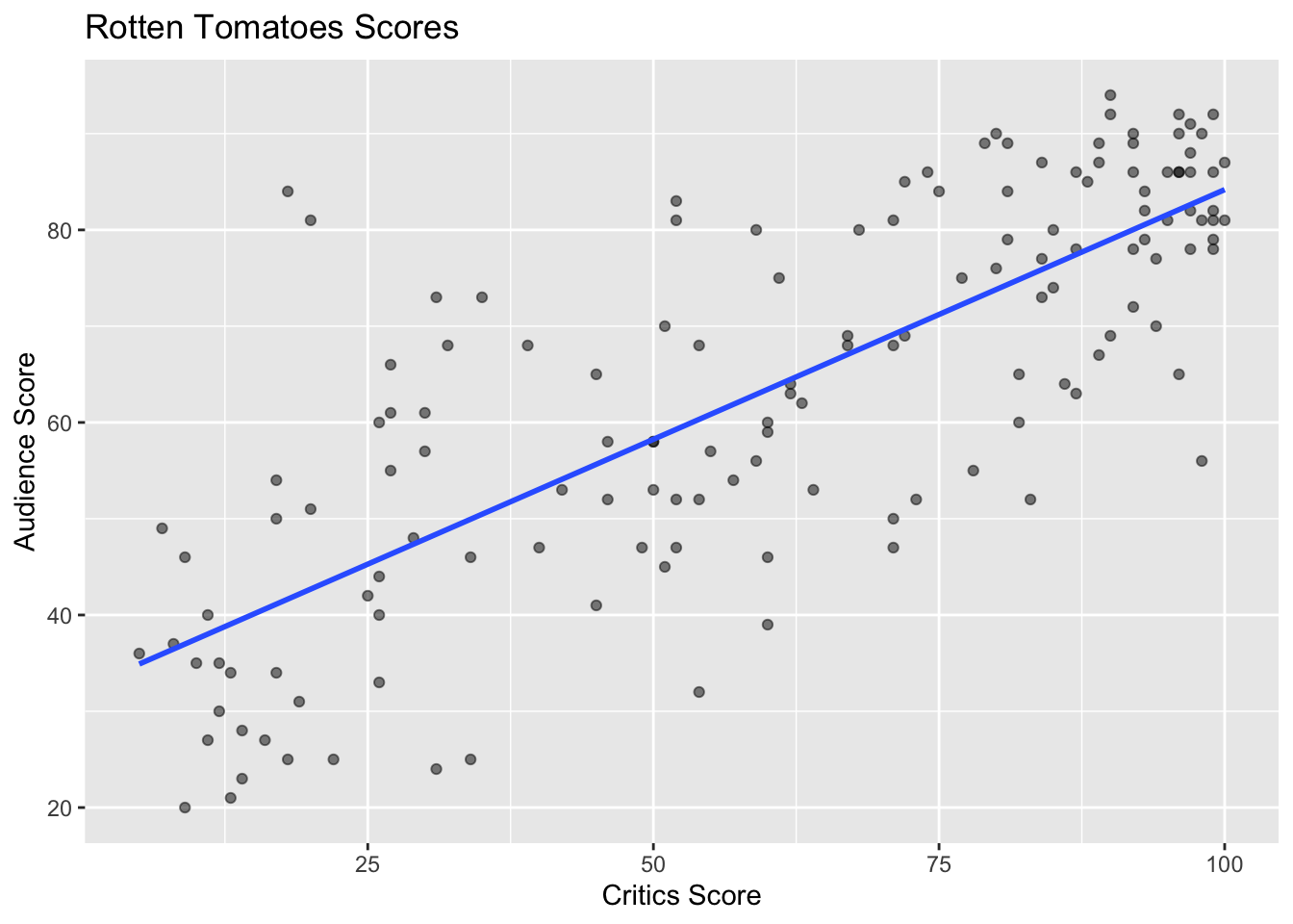
Recap: simple linear regression

Numerical response and one numerical predictor:

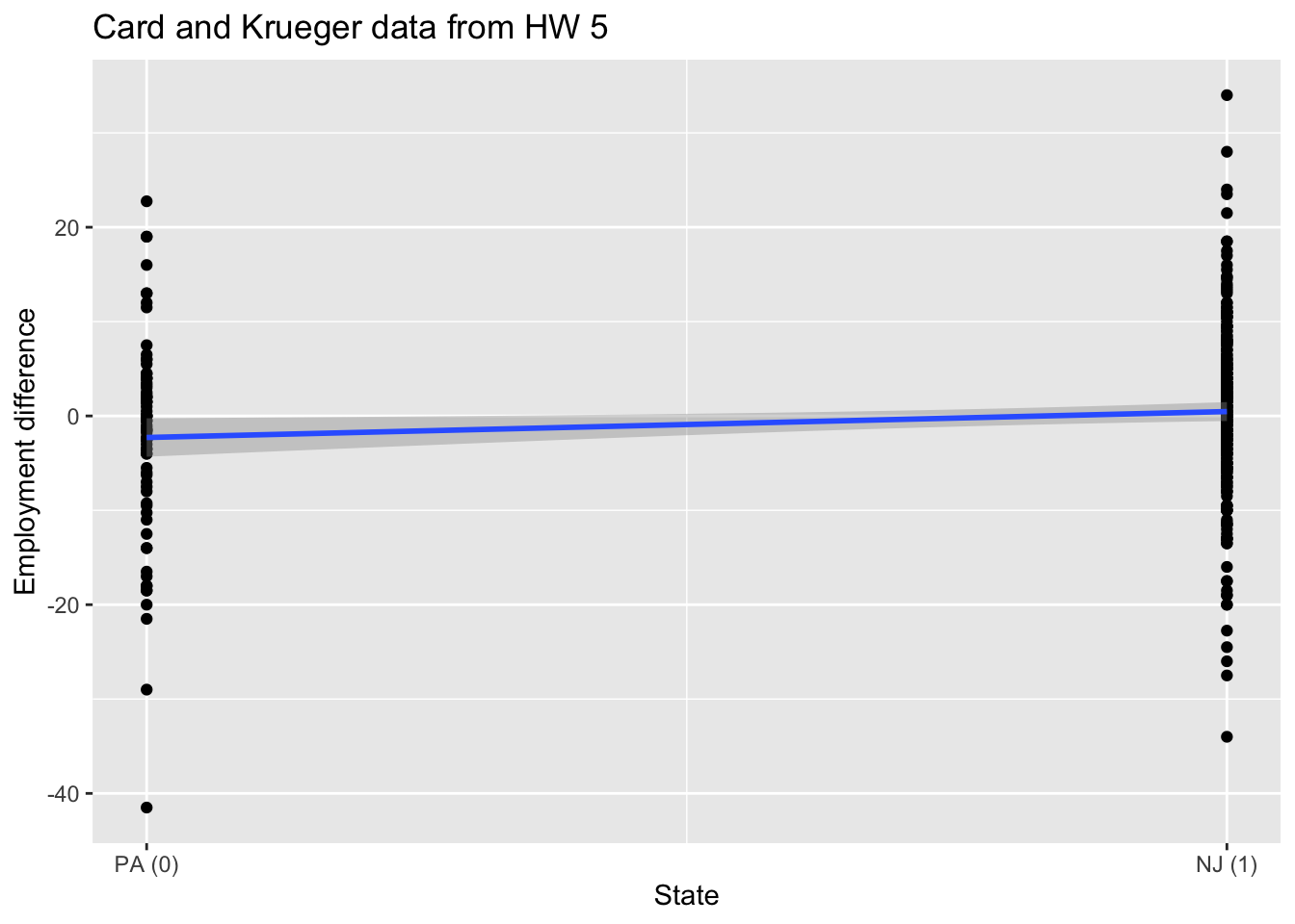
Recap: simple linear regression

Numerical response and one categorical predictor (two levels):

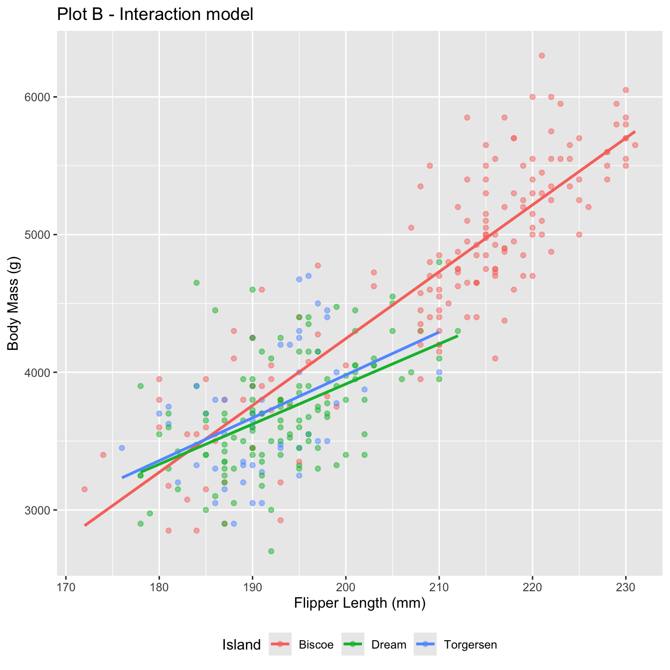
Recap: multiple linear regression

Numerical response; numerical and categorical predictors:

`geom_smooth()` using formula = 'y ~ x'

Warning: Removed 2 rows containing non-finite outside the scale range
(`stat_smooth()`).

Warning: Removed 2 rows containing missing values or values outside the scale range
(`geom_point()`).

`geom_smooth()` using formula = 'y ~ x'

Warning: Removed 2 rows containing non-finite outside the scale range (`stat_smooth()`).
Removed 2 rows containing missing values or values outside the scale range
(`geom_point()`).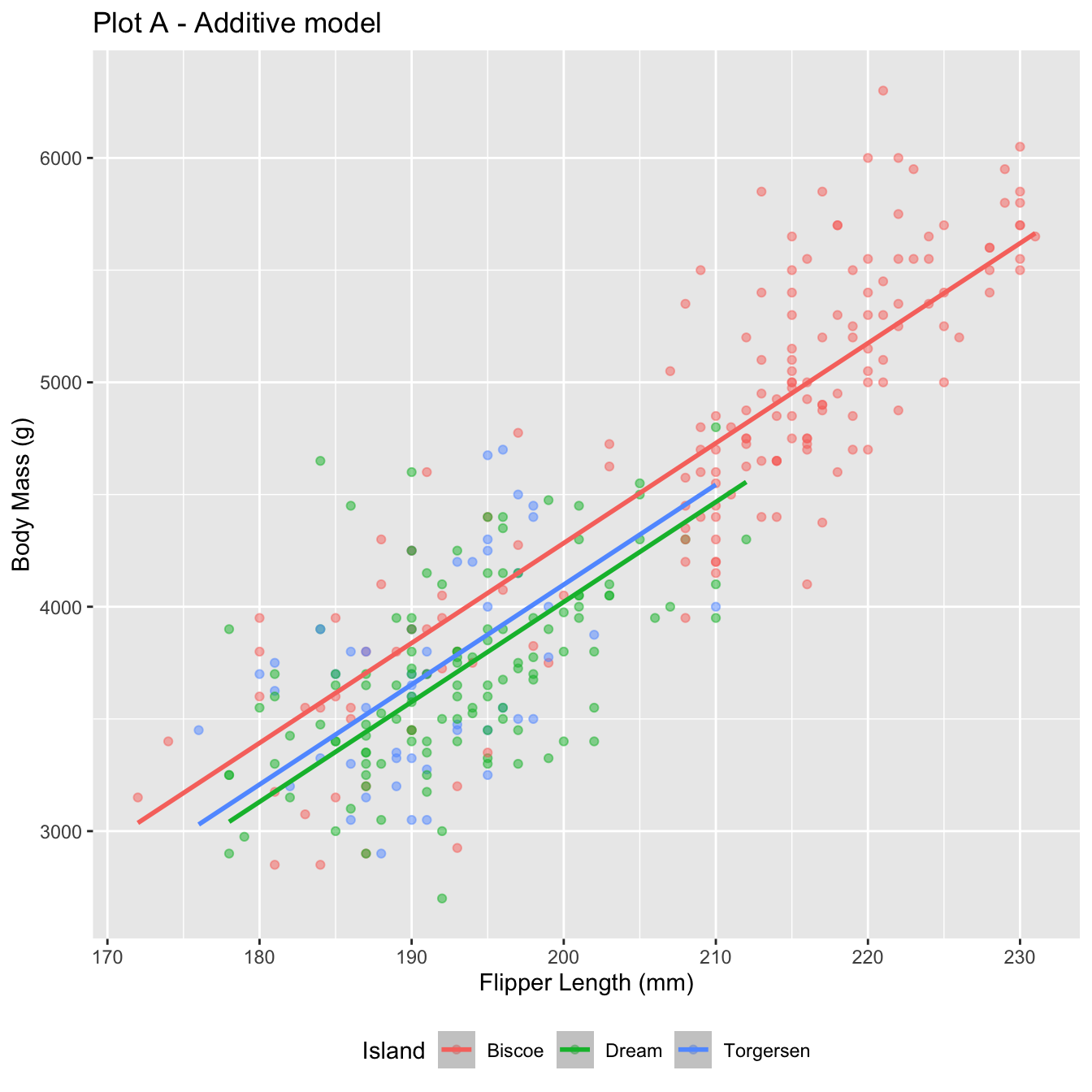

Today: a binary response

\[ y = \begin{cases} 1 & &&\text{eg. Yes, Win, True, Heads, Success}\\ 0 & &&\text{eg. No, Lose, False, Tails, Failure}. \end{cases} \]

Who cares?

If we can model the relationship between predictors (\(x\)) and a binary response (\(y\)), we can use the model to do a special kind of prediction called classification.

Example: is the e-mail spam or not?

\[ \mathbf{x}: \text{word and character counts in an e-mail.} \]

\[ y = \begin{cases} 1 & \text{it's spam}\\ 0 & \text{it's legit} \end{cases} \]

Example: is it cancer or not?

\[ \mathbf{x}: \text{features in a medical image.} \]

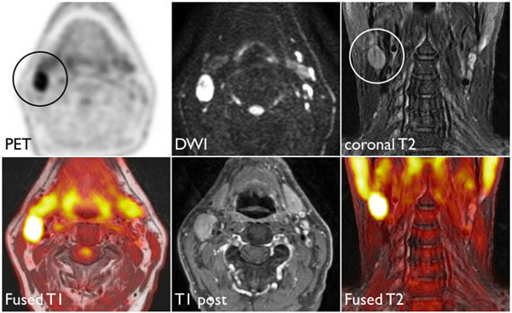
\[ y = \begin{cases} 1 & \text{it's cancer}\\ 0 & \text{it's healthy} \end{cases} \]

Example: will they default?

\[ \mathbf{x}: \text{financial and demographic info about a loan applicant.} \]

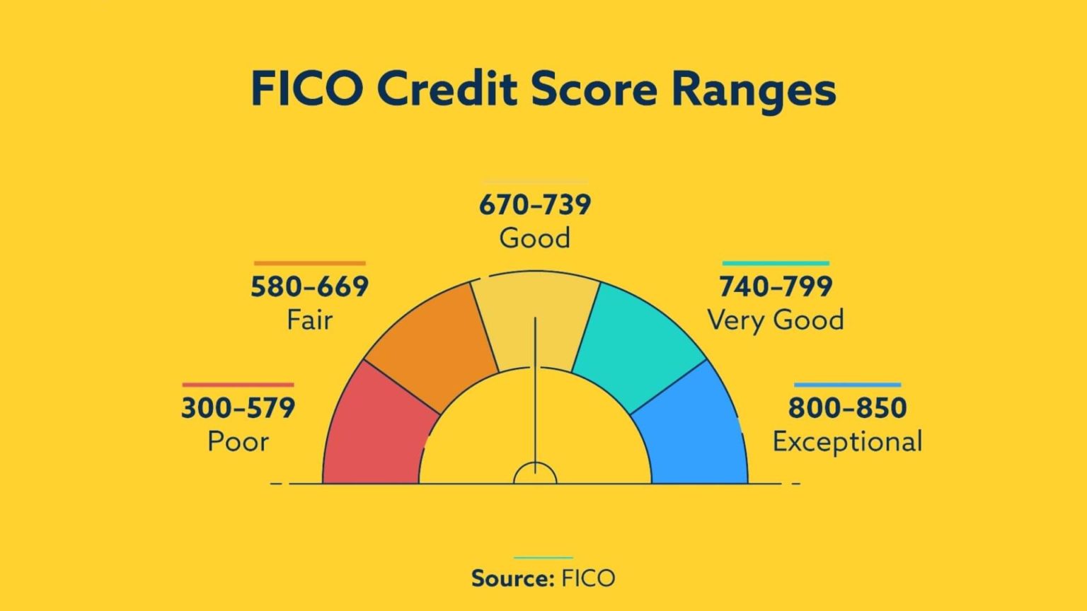
\[ y = \begin{cases} 1 & \text{applicant is at risk of defaulting on loan}\\ 0 & \text{applicant is safe} \end{cases} \]

Example: Who said it: Taylor Swift, or Shakespeare?

\[ \mathbf{x}: \text{word counts (e.g., thou, love, heartbreak), stylistic features} \]

\[ y = \begin{cases} 1 & \text{Taylor Swift}\\ 0 & \text{William Shakespeare} \end{cases} \]

How do we model this type of data?

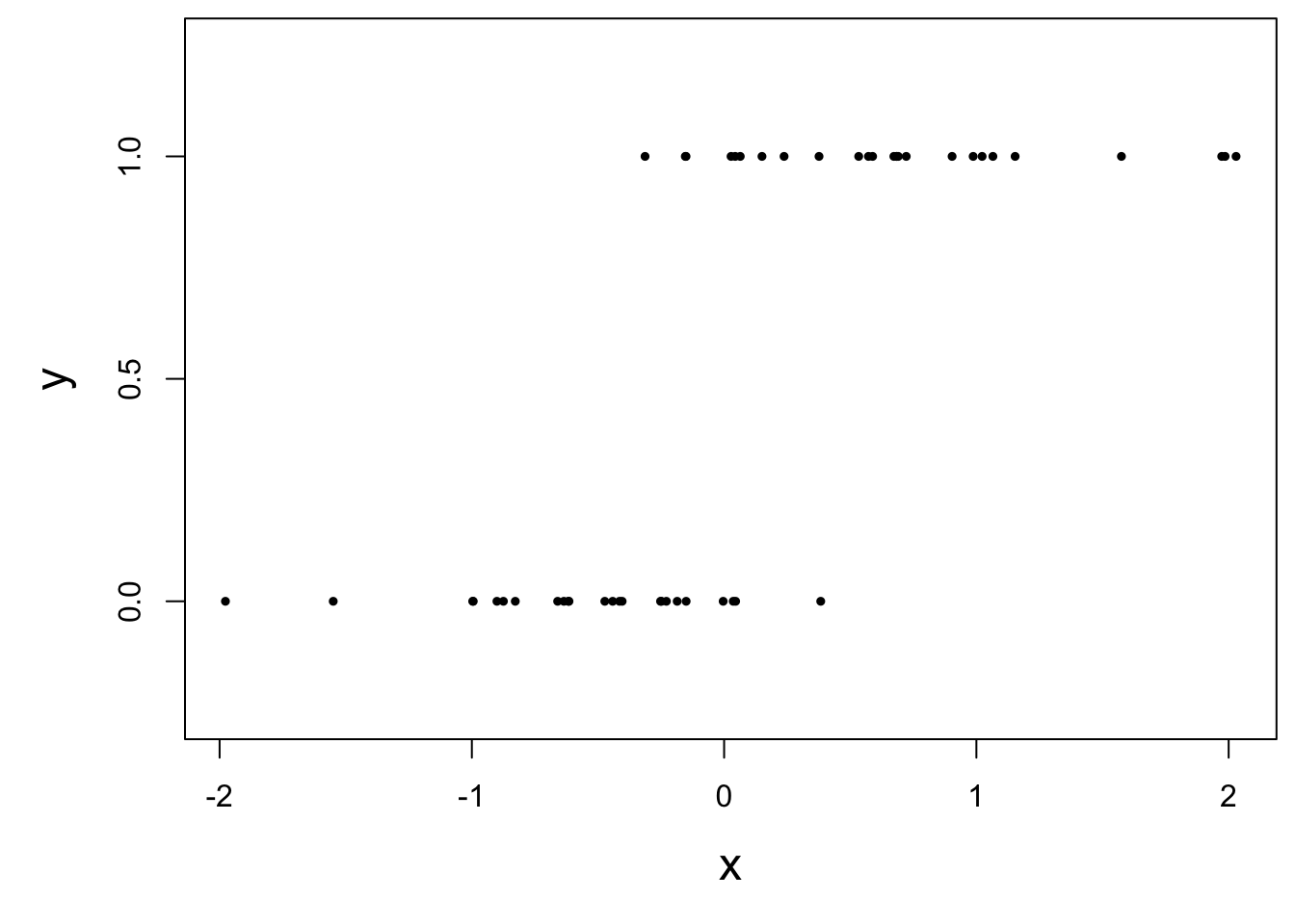
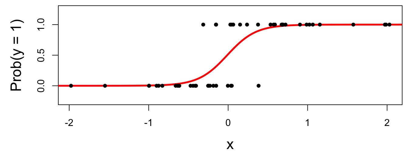
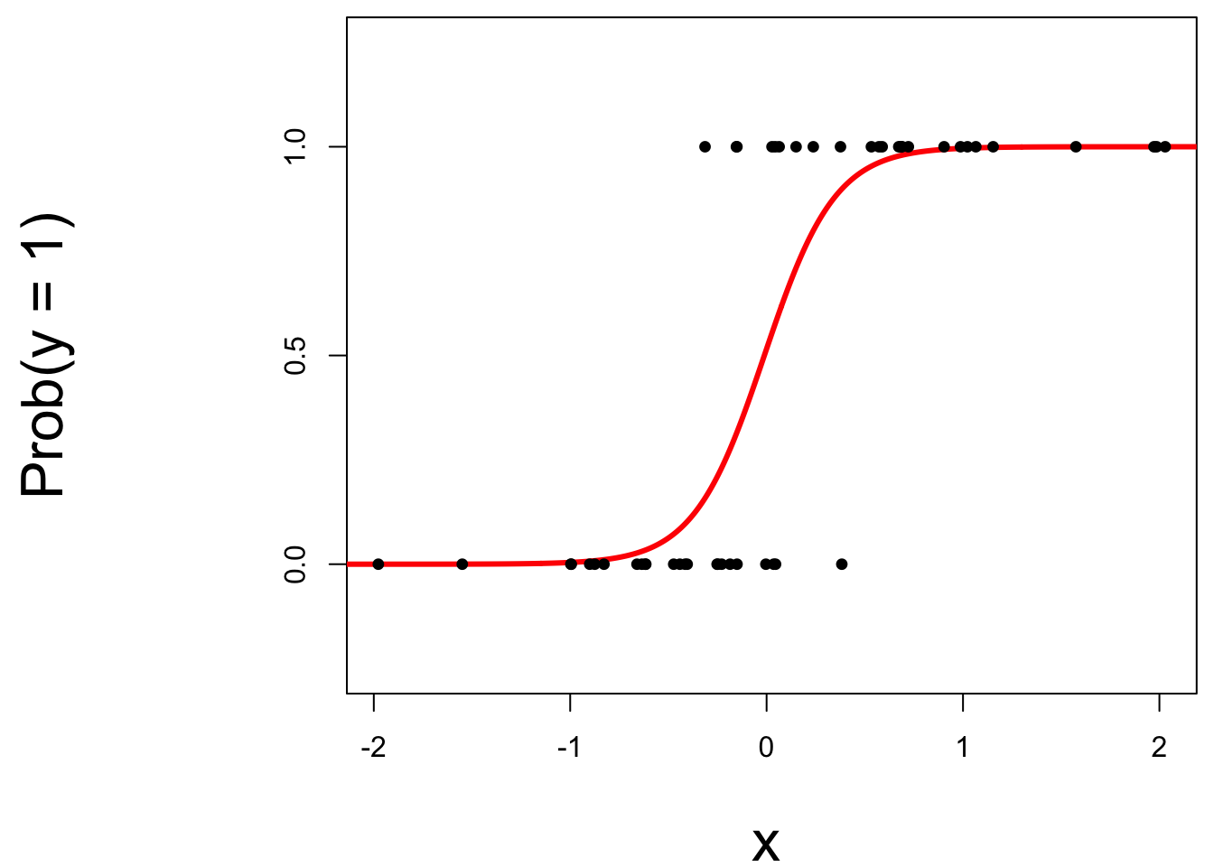
Straight line of best fit is a little silly

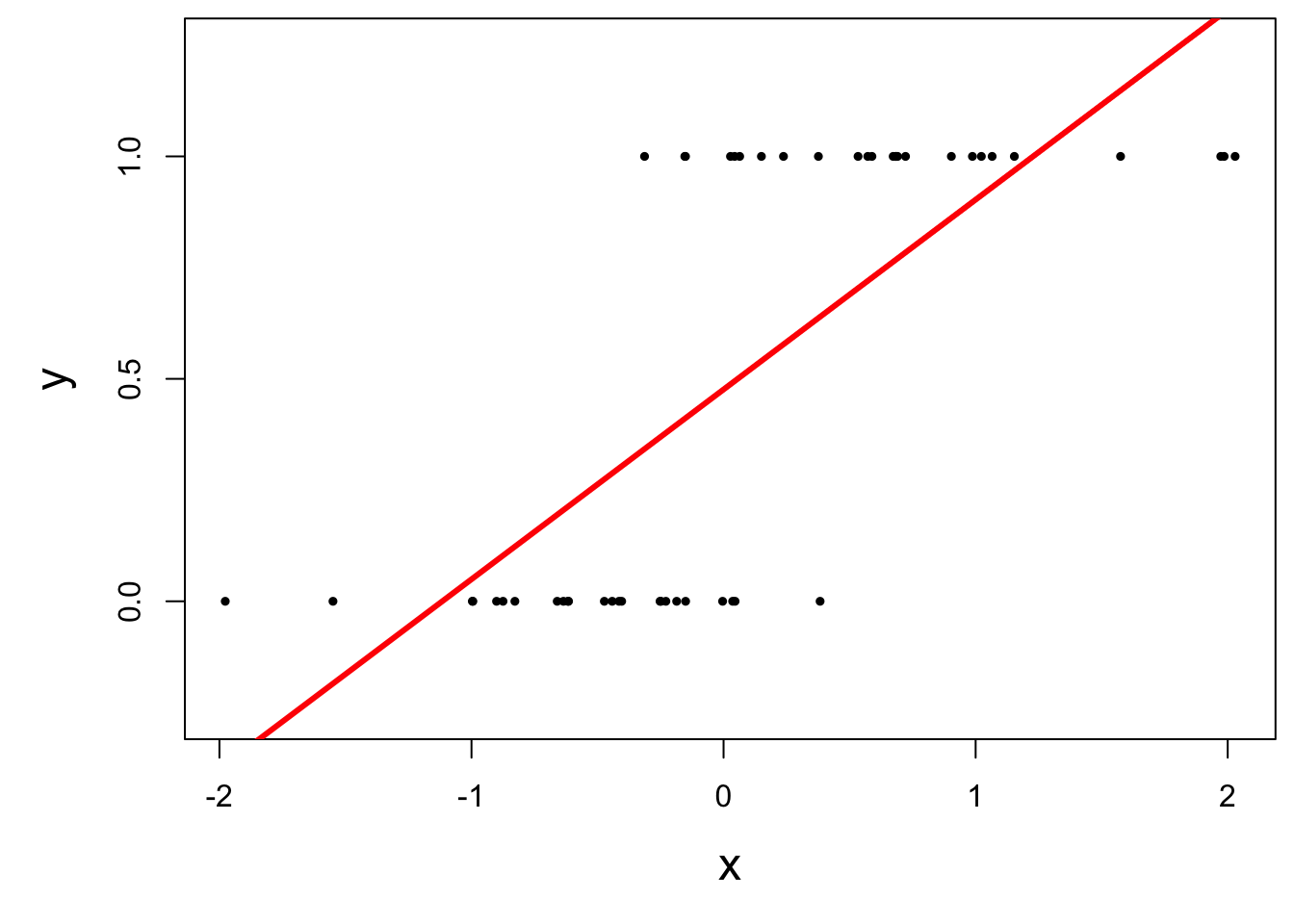
Instead: S-curve of best fit

Instead of modeling \(y\) directly, we model the probability that \(y=1\):

“Given new email, what’s the probability that it’s spam?’’
“Given new image, what’s the probability that it’s cancer?’’
“Given new loan application, what’s the probability that they default?’’

Why don’t we model y directly?

Recall regression with a numerical response:
- Our models do not output guarantees for \(y\), they output predictions that describe behavior on average;
Similar when modeling a binary response:
- Our models cannot directly guarantee that \(y\) will be zero or one. The correct analog to “on average” for a 0/1 response is “what’s the probability?”

So, what is this S-curve, anyway?

It’s the logistic function:

\[ \text{Prob}(y = 1) = \frac{e^{\beta_0+\beta_1x}}{1+e^{\beta_0+\beta_1x}}. \]

If you set \(p = \text{Prob}(y = 1)\) and do some algebra, you get the simple linear model for the log-odds:

\[ \log\left(\frac{p}{1-p}\right) = \beta_0+\beta_1x. \]

This is called the logistic regression model.

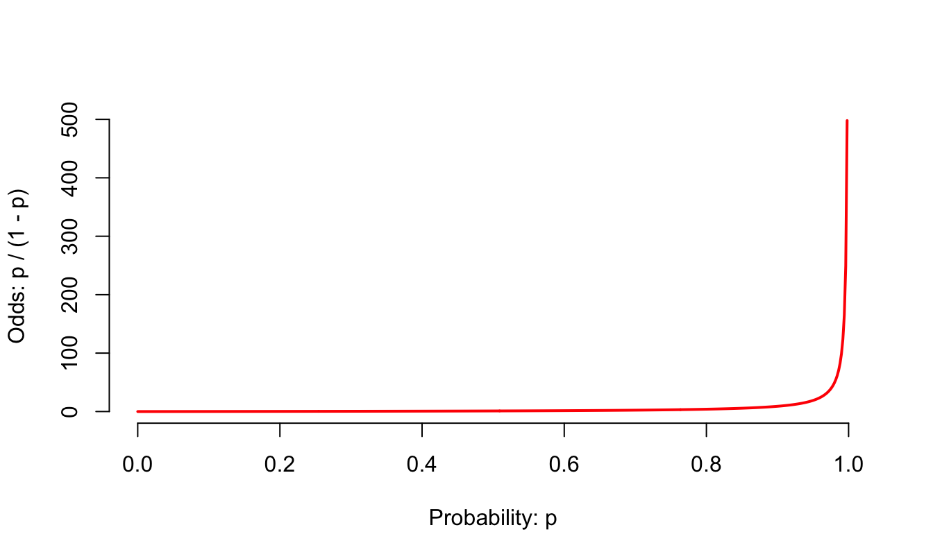
Log-odds?

\(p = \text{Prob}(y = 1)\) is a probability. A number between 0 and 1;
\(p / (1 - p)\) is the odds. A number between 0 and \(\infty\);

“The odds of this lecture going well are 10 to 1.”

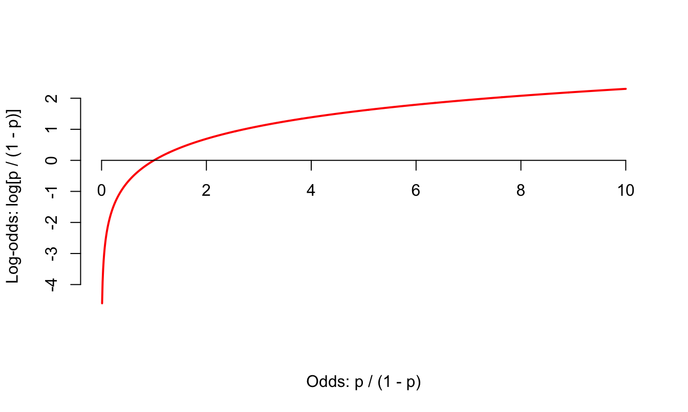
The log odds \(\log(p / (1 - p))\) is a number between \(-\infty\) and \(\infty\), which is suitable for the linear model.
Why does this “transformation” work? The log function maps positive numbers \((0, \infty)\) to all real numbers \((-\infty, \infty)\).

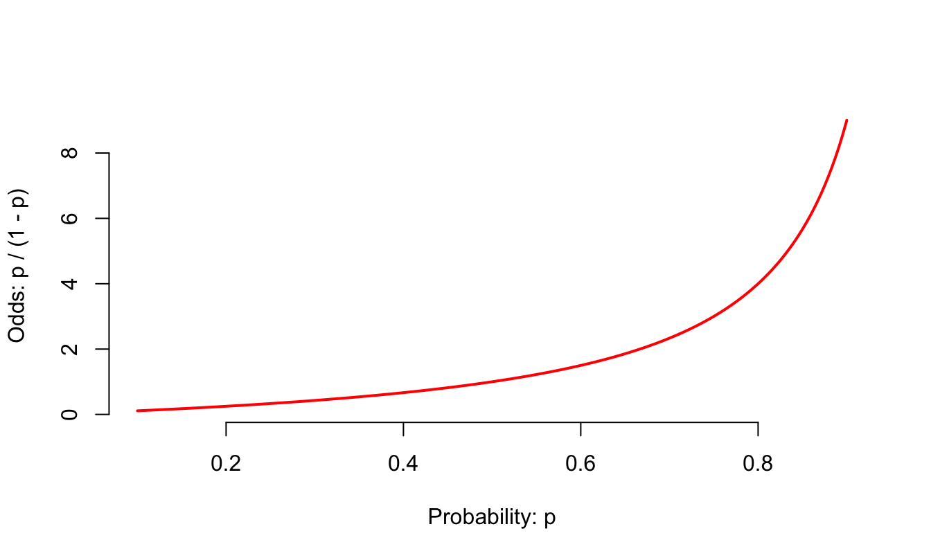
Probability to odds

Zooming in

Odds to log odds

Logistic regression

\[ \log\left(\frac{p}{1-p}\right) = \beta_0+\beta_1x. \]

The logit function \(\log(p / (1-p))\) is an example of a link function that transforms the linear model to have an appropriate range;
This is an example of a generalized linear model

Estimation

We estimate the parameters \(\beta_0,\,\beta_1\) using maximum likelihood (don’t worry about it) to get the “best fitting” S-curve;
The fitted model is

\[ \log\left(\frac{\widehat{p}}{1-\widehat{p}}\right) = b_0+b_1x. \]

Today’s data

email |> 
  dplyr::select(c(spam, dollar, viagra, winner, password, exclaim_mess)) |> 
  glimpse()

Rows: 3,921
Columns: 6
$ spam         <fct> 0, 0, 0, 0, 0, 0, 0, 0, 0, 0, 0, 0, 0, 0, 0, 0, 0, 0, 0, …
$ dollar       <dbl> 0, 0, 4, 0, 0, 0, 0, 0, 0, 0, 0, 0, 0, 0, 2, 0, 5, 0, 0, …
$ viagra       <dbl> 0, 0, 0, 0, 0, 0, 0, 0, 0, 0, 0, 0, 0, 0, 0, 0, 0, 0, 0, …
$ winner       <fct> no, no, no, no, no, no, no, no, no, no, no, no, no, no, n…
$ password     <dbl> 0, 0, 0, 0, 2, 2, 0, 0, 0, 0, 0, 0, 0, 0, 0, 0, 1, 0, 0, …
$ exclaim_mess <dbl> 0, 1, 6, 48, 1, 1, 1, 18, 1, 0, 2, 1, 0, 10, 4, 10, 20, 0…

Fitting a logistic model

logistic_fit <- logistic_reg() |>
  fit(spam ~ exclaim_mess, data = email)

tidy(logistic_fit)

# A tibble: 2 × 5
  term          estimate std.error statistic p.value
  <chr>            <dbl>     <dbl>     <dbl>   <dbl>
1 (Intercept)  -2.27      0.0553     -41.1     0    
2 exclaim_mess  0.000272  0.000949     0.287   0.774

Fitted equation for the log-odds:

\[ \log\left(\frac{\hat{p}}{1-\hat{p}}\right) = -2.27 + 0.000272\times exclaim~mess \]

Interpreting the intercept

If exclaim_mess = 0, then

\[ \hat{p}=\widehat{P(y=1)}=\frac{e^{-2.27}}{1+e^{-2.27}}\approx 0.09. \]

So, our model predicts that an email with no exclamation marks has a 9% probability of being spam.

Participate 📱💻

The slope of the logistic regression model for these data is 0.000272. Which of the following is the best interpretation of this value?

If we add one exclamation mark to the model, we predict the probability of an email being spam will increase by 0.000272, on average.
If we add one exclamation mark to the model, we predict the odds of an email being spam will increase by 0.000272, on average.
If we add one exclamation mark to the model, we predict the odds of an email being spam to be higher by a factor of e^0.000272 = 1.000272, on average.
The odds of an email being spam are decreasing in the number of exclamation marks.

Scan the QR code or go HERE. Log in with your Duke NetID.

Interpreting the slope is tricky

Recall:

\[ \log\left(\frac{\widehat{p}}{1-\widehat{p}}\right) = b_0+b_1x. \]

. . .

Alternatively:

\[ \frac{\widehat{p}}{1-\widehat{p}} = e^{b_0+b_1x} = \color{blue}{e^{b_0}e^{b_1x}} . \]

. . .

If we increase \(x\) by one unit, we have:

\[ \frac{\widehat{p}}{1-\widehat{p}} = e^{b_0}e^{b_1(x+1)} = e^{b_0}e^{b_1x+b_1} = {\color{blue}{e^{b_0}e^{b_1x}}}{\color{red}{e^{b_1}}} . \]

. . .

A one unit increase in \(x\) is associated with a change in odds by a factor of \(e^{b_1}\). Gross!

Back to the example…

\[ \log\left(\frac{\hat{p}}{1-\hat{p}}\right) = -2.27 + 0.000272\times exclaim~mess \]

If the email has an additional exclamation mark, we predict the odds of an email being spam to be higher by a multiplicative factor of \(e^{0.000272}\approx 1.000272\) on average.

Logistic regression -> classification?

Step 0: fit the model

Select a number \(0 < p^* < 1\):

if \(\text{Prob}(y=1)\leq p^*\), then predict \(\widehat{y}=0\);
if \(\text{Prob}(y=1)> p^*\), then predict \(\widehat{y}=1\).

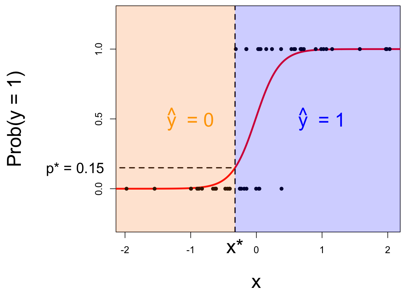
Step 1: pick a threshold

Select a number \(0 < p^* < 1\):

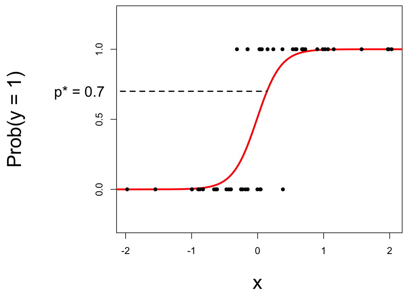
if \(\text{Prob}(y=1)\leq p^*\), then predict \(\widehat{y}=0\);
if \(\text{Prob}(y=1)> p^*\), then predict \(\widehat{y}=1\).

Step 2: find the “decision boundary”

Solve for the x-value that matches the threshold:

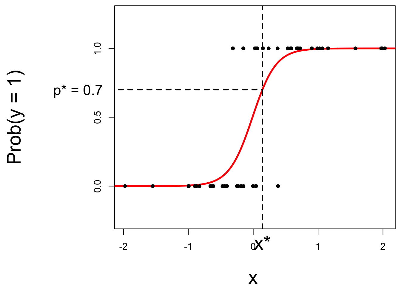
if \(\text{Prob}(y=1)\leq p^*\), then predict \(\widehat{y}=0\);
if \(\text{Prob}(y=1)> p^*\), then predict \(\widehat{y}=1\).

Step 3: classify a new arrival

A new person shows up with \(x_{\text{new}}\). Which side of the boundary are they on?

if \(x_{\text{new}} \leq x^\star\), then \(\text{Prob}(y=1)\leq p^*\), so predict \(\widehat{y}=0\) for the new person;
if \(x_{\text{new}} > x^\star\), then \(\text{Prob}(y=1)> p^*\), so predict \(\widehat{y}=1\) for the new person.

Let’s change the threshold

A new person shows up with \(x_{\text{new}}\). Which side of the boundary are they on?

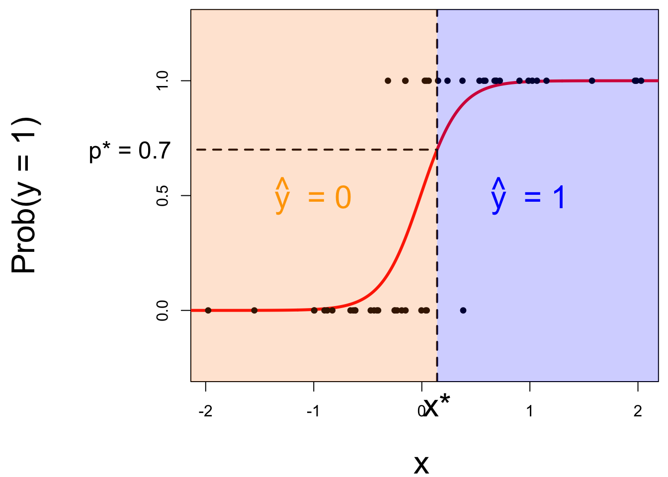
if \(x_{\text{new}} \leq x^\star\), then \(\text{Prob}(y=1)\leq p^*\), so predict \(\widehat{y}=0\) for the new person;
if \(x_{\text{new}} > x^\star\), then \(\text{Prob}(y=1)> p^*\), so predict \(\widehat{y}=1\) for the new person.

Let’s change the threshold

A new person shows up with \(x_{\text{new}}\). Which side of the boundary are they on?

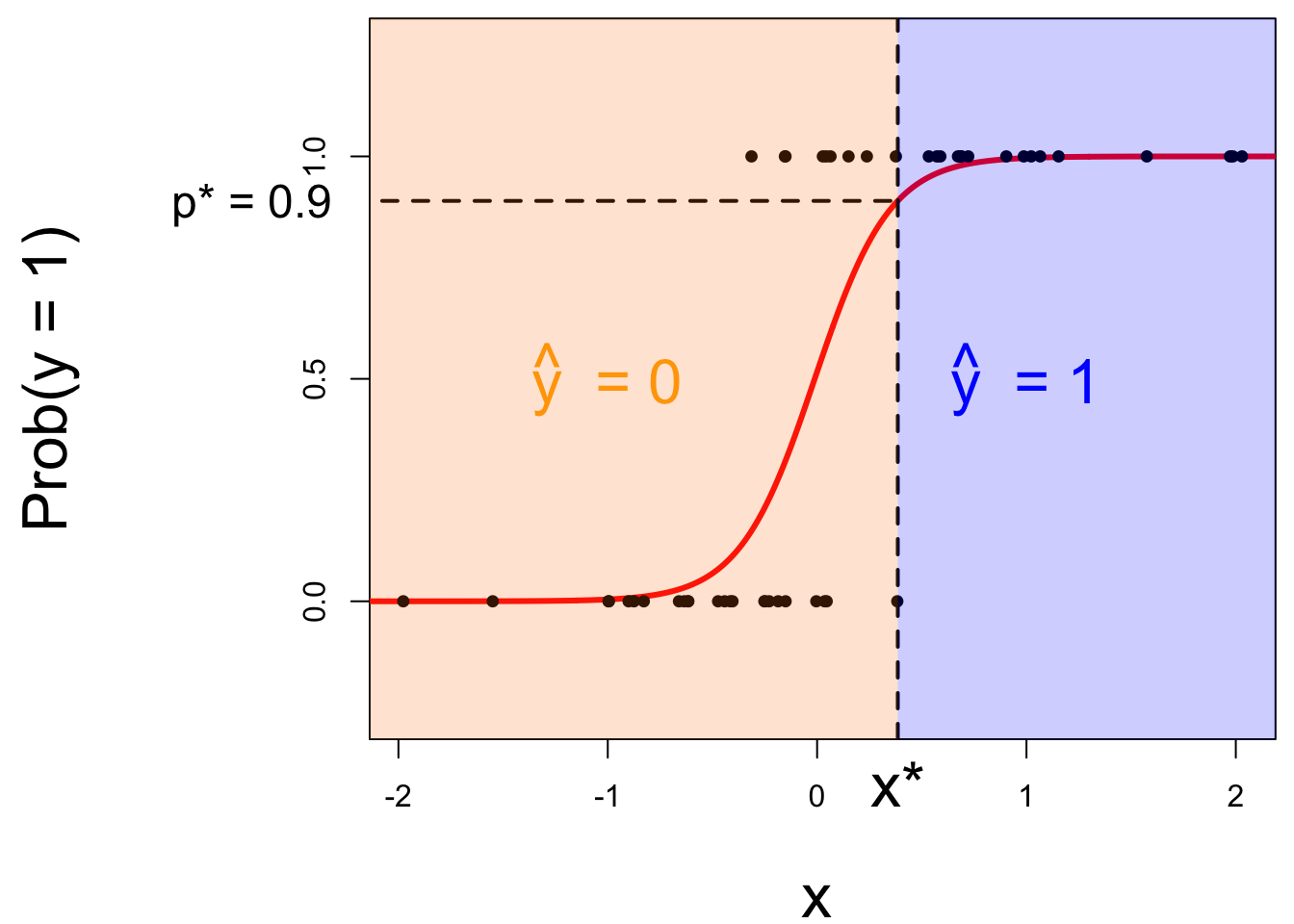
if \(x_{\text{new}} \leq x^\star\), then \(\text{Prob}(y=1)\leq p^*\), so predict \(\widehat{y}=0\) for the new person;
if \(x_{\text{new}} > x^\star\), then \(\text{Prob}(y=1)> p^*\), so predict \(\widehat{y}=1\) for the new person.

Nothing special about one predictor…

Two numerical predictors and one binary response:

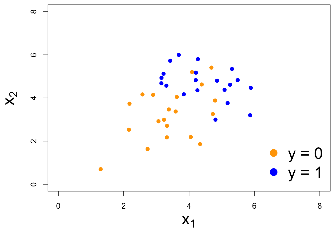
“Multiple” logistic regression

For the log-odds, a multiple linear regression:

\[ \log\left(\frac{p}{1-p}\right) = \beta_0+\beta_1x_1+\beta_2x_2+...+\beta_mx_m. \] On the probability scale:

\[ \text{Prob}(y = 1) = \frac{e^{\beta_0+\beta_1x_1+\beta_2x_2+...+\beta_mx_m}}{1+e^{\beta_0+\beta_1x_1+\beta_2x_2+...+\beta_mx_m}}. \]

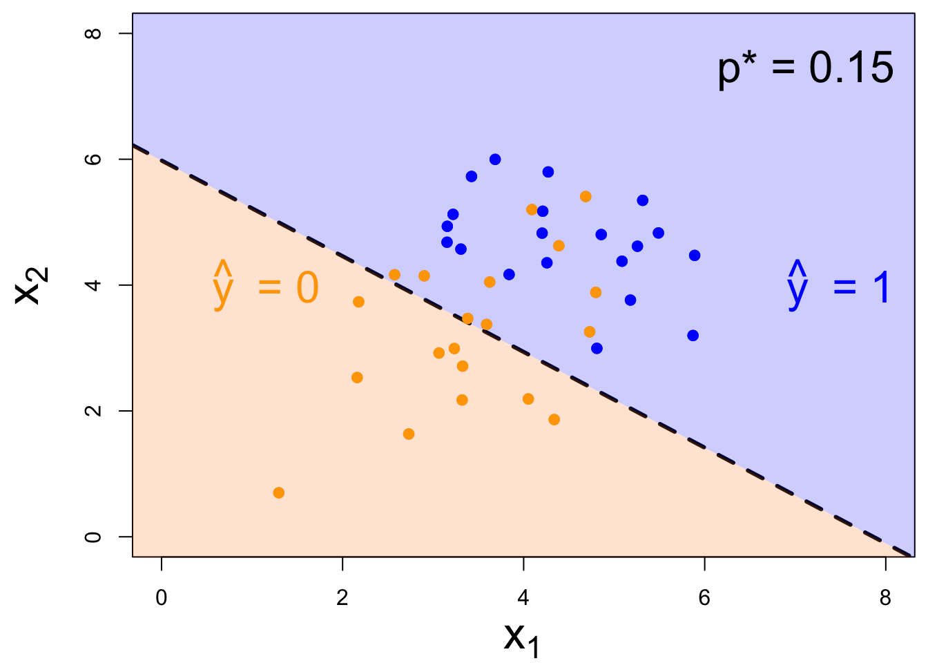
Decision boundary, again

It’s linear! Consider two numerical predictors:

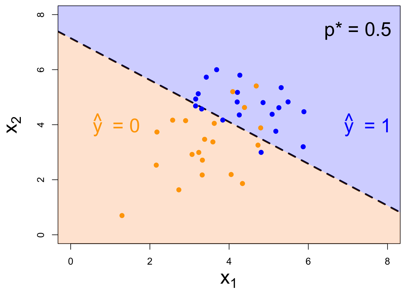
if new \((x_1,\,x_2)\) below, \(\text{Prob}(y=1)\leq p^*\). Predict \(\widehat{y}=0\) for the new person;
if new \((x_1,\,x_2)\) above, \(\text{Prob}(y=1)> p^*\). Predict \(\widehat{y}=1\) for the new person.

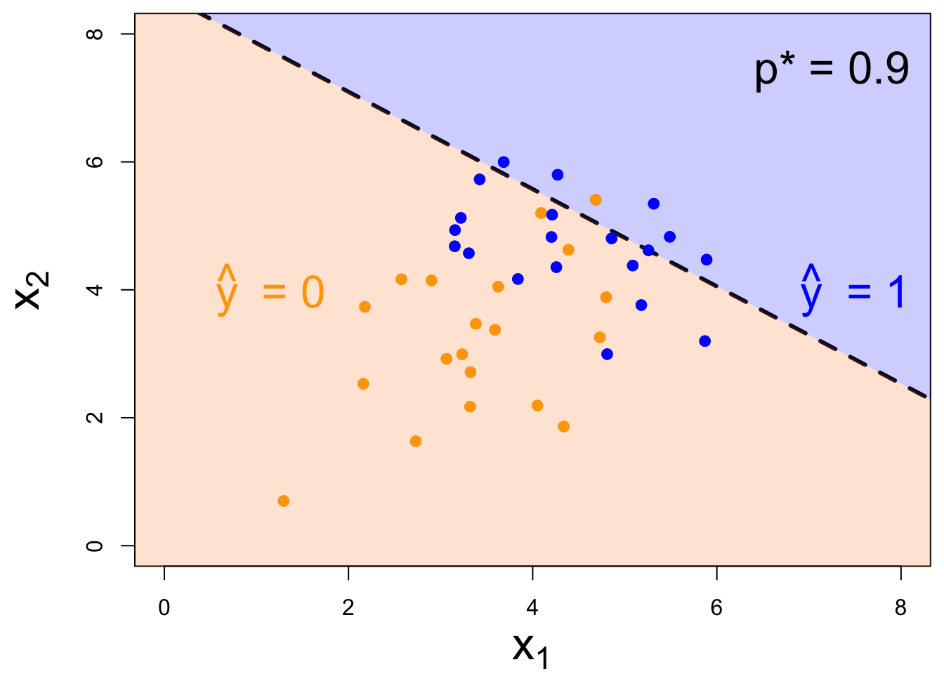
Decision boundary, again

It’s linear! Consider two numerical predictors:

if new \((x_1,\,x_2)\) below, \(\text{Prob}(y=1)\leq p^*\). Predict \(\widehat{y}=0\) for the new person;
if new \((x_1,\,x_2)\) above, \(\text{Prob}(y=1)> p^*\). Predict \(\widehat{y}=1\) for the new person.

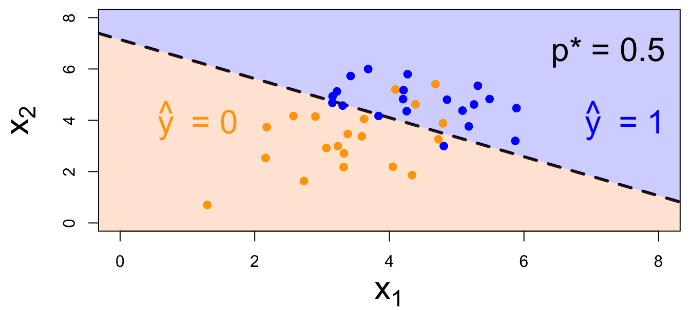
Decision boundary, again

It’s linear! Consider two numerical predictors:

if new \((x_1,\,x_2)\) below, \(\text{Prob}(y=1)\leq p^*\). Predict \(\widehat{y}=0\) for the new person;
if new \((x_1,\,x_2)\) above, \(\text{Prob}(y=1)> p^*\). Predict \(\widehat{y}=1\) for the new person.

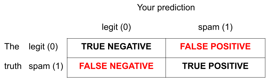
Note: the classifier isn’t perfect

There are blue points in the orange region: spam (1) emails misclassified as legit (0);
There are orange points in the blue region: legit (0) emails misclassified as spam (1).

How do you pick the threshold?

To balance out the two kinds of errors:

High threshold >> Hard to classify as 1 >> FP less likely; FN more likely
Low threshold >> Easy to classify as 1 >> FP more likely; FN less likely

Silly examples

Set p* = 0
- Classify every email as spam (1);
- No false negatives, but a lot of false positives;
Set p* = 1
- Classify every email as legit (0);
- No false positives, but a lot of false negatives.

You pick a threshold in between to strike a balance. The exact number depends on context.

ae-19-spam-filter

Go to your ae project in RStudio.
If you haven’t yet done so, make sure all of your changes up to this point are committed and pushed, i.e., there’s nothing left in your Git pane.
If you haven’t yet done so, click Pull to get today’s application exercise file: ae-19-spam-filter.qmd.
Work through the application exercise in class, and render, commit, and push your edits.