Rows: 7,107
Columns: 20
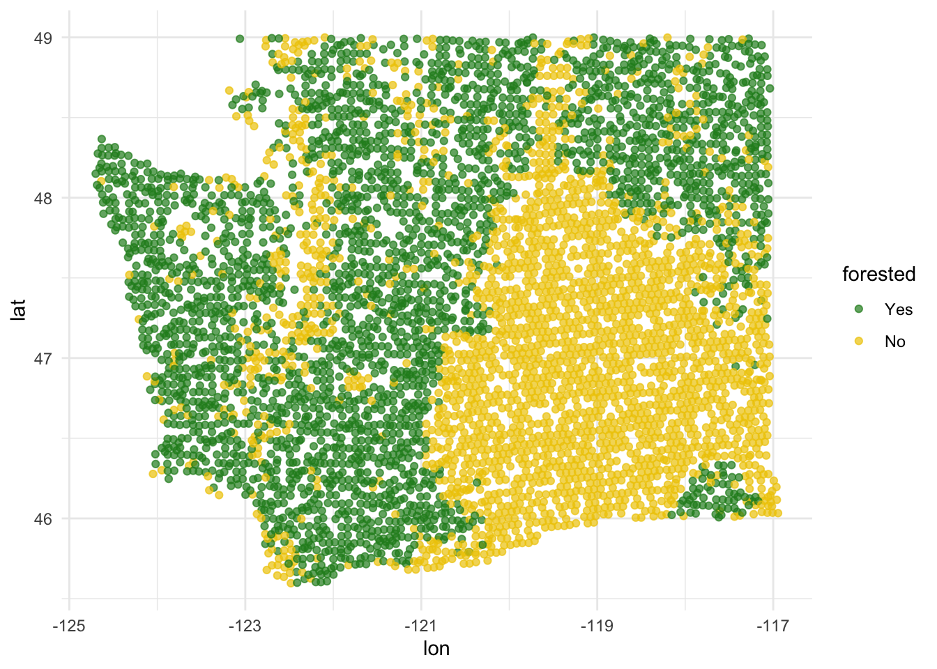
$ forested <fct> Yes, Yes, No, Yes, Yes, Yes, Yes, Yes, Yes, Yes, Yes,…
$ year <dbl> 2005, 2005, 2005, 2005, 2005, 2005, 2005, 2005, 2005,…
$ elevation <dbl> 881, 113, 164, 299, 806, 736, 636, 224, 52, 2240, 104…
$ eastness <dbl> 90, -25, -84, 93, 47, -27, -48, -65, -62, -67, 96, -4…
$ northness <dbl> 43, 96, 53, 34, -88, -96, 87, -75, 78, -74, -26, 86, …
$ roughness <dbl> 63, 30, 13, 6, 35, 53, 3, 9, 42, 99, 51, 190, 95, 212…
$ tree_no_tree <fct> Tree, Tree, Tree, No tree, Tree, Tree, No tree, Tree,…
$ dew_temp <dbl> 0.04, 6.40, 6.06, 4.43, 1.06, 1.35, 1.42, 6.39, 6.50,…
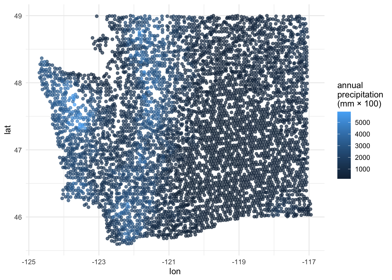
$ precip_annual <dbl> 466, 1710, 1297, 2545, 609, 539, 702, 1195, 1312, 103…
$ temp_annual_mean <dbl> 6.42, 10.64, 10.07, 9.86, 7.72, 7.89, 7.61, 10.45, 10…
$ temp_annual_min <dbl> -8.32, 1.40, 0.19, -1.20, -5.98, -6.00, -5.76, 1.11, …
$ temp_annual_max <dbl> 12.91, 15.84, 14.42, 15.78, 13.84, 14.66, 14.23, 15.3…
$ temp_january_min <dbl> -0.08, 5.44, 5.72, 3.95, 1.60, 1.12, 0.99, 5.54, 6.20…
$ vapor_min <dbl> 78, 34, 49, 67, 114, 67, 67, 31, 60, 79, 172, 162, 70…
$ vapor_max <dbl> 1194, 938, 754, 1164, 1254, 1331, 1275, 944, 892, 549…
$ canopy_cover <dbl> 50, 79, 47, 42, 59, 36, 14, 27, 82, 12, 74, 66, 83, 6…
$ lon <dbl> -118.6865, -123.0825, -122.3468, -121.9144, -117.8841…
$ lat <dbl> 48.69537, 47.07991, 48.77132, 45.80776, 48.07396, 48.…
$ land_type <fct> Tree, Tree, Tree, Tree, Tree, Tree, Non-tree vegetati…
$ county <fct> Ferry, Thurston, Whatcom, Skamania, Stevens, Stevens,…Logistic regression 3
Lecture 21
2026-04-06
Wednesday: SSMU Talk
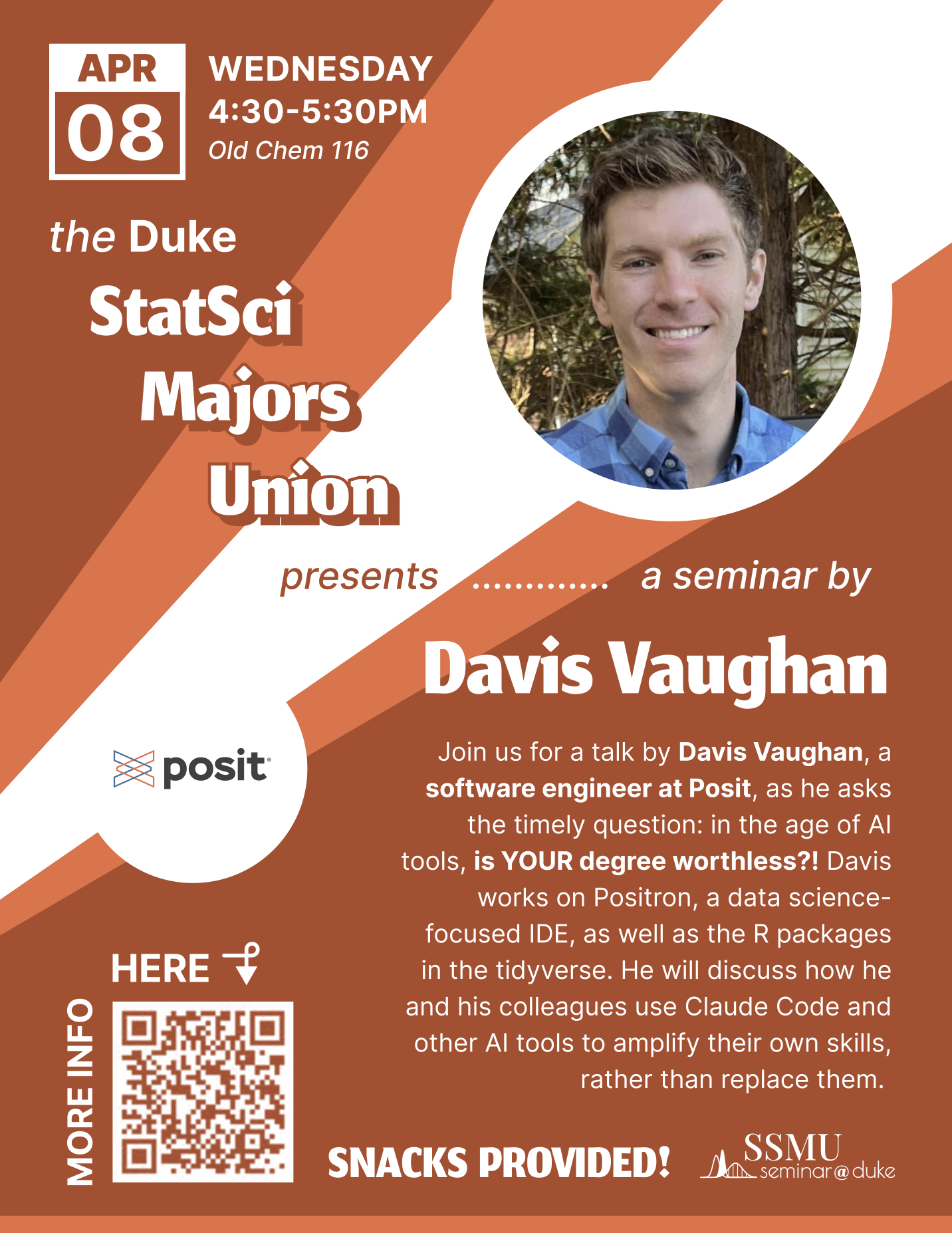
- The old broads in the stats mafia host an even older broad from the tidy mafia to scare you about your future
- Wednesday April 8 @ 4:30 pm
- Old Chem 116
Wednesday: Duke Symphony Concert

- Duke Symphony Orchestra
- Wednesday April 8 @ 7:30 pm
- Baldwin Auditorium (East Campus)
- WANANA classmates and TAs!
Thursday: Six Characters in Search of an Author
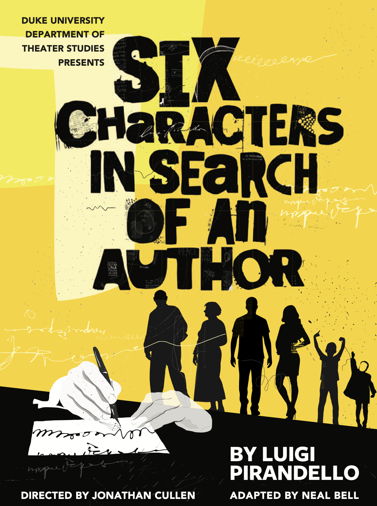
- Play by Luigi Pirandello
- April 9 - 11 @ 8 p.m
- April 12 @ 2pm
- Sheafer Lab Theater here in Bryan Center
Friday: Duke Chinese Dance

- Insta: @dukechinesedance
- Friday April 10 @ 7pm
- Page Auditorium
- Classmates! TAs! Josh!
Friday: Momentum Showcase
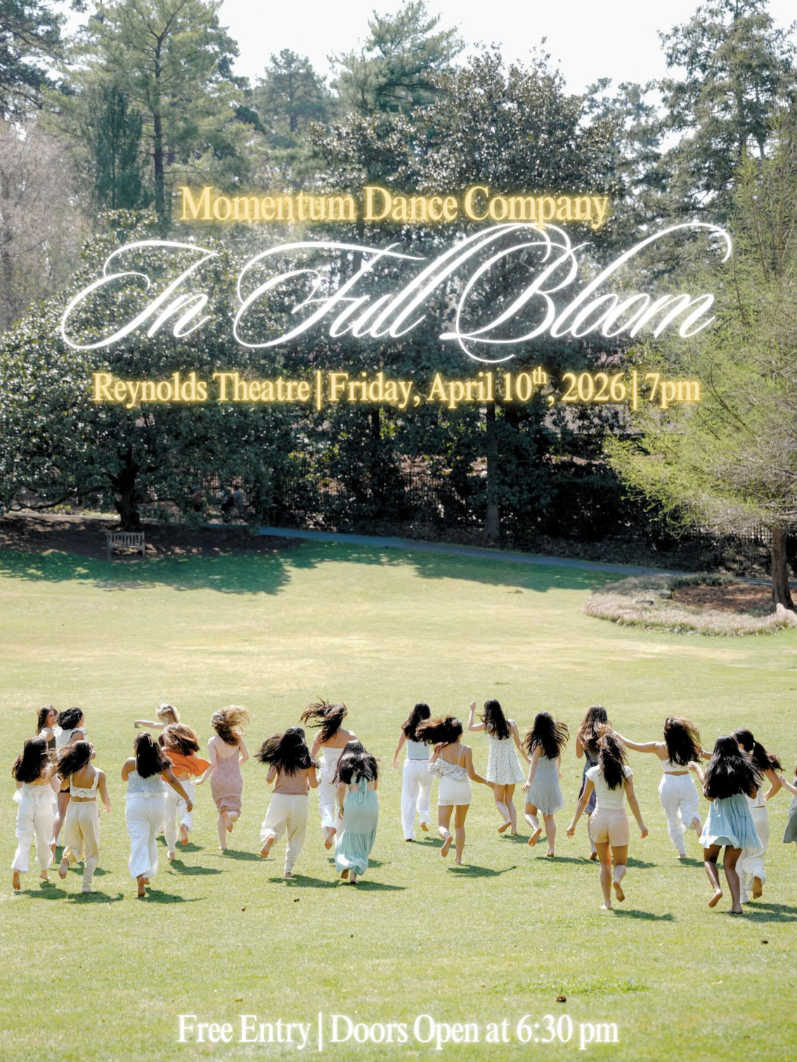
- Insta: @momentum_duke
- Friday April 10 @ 7pm
- Reynolds Theatre
- Lily! Katarina!
Saturday: DBBH’s Spring Business Conference

- Duke Business Behind Health (DBBH)
- Saturday April 11
- In the business school
- Great if you’re pre-med, pre-biotech, etc
- Rub elbows with the muckety-mucks!
Saturday: Devils en Pointe and Embodiment
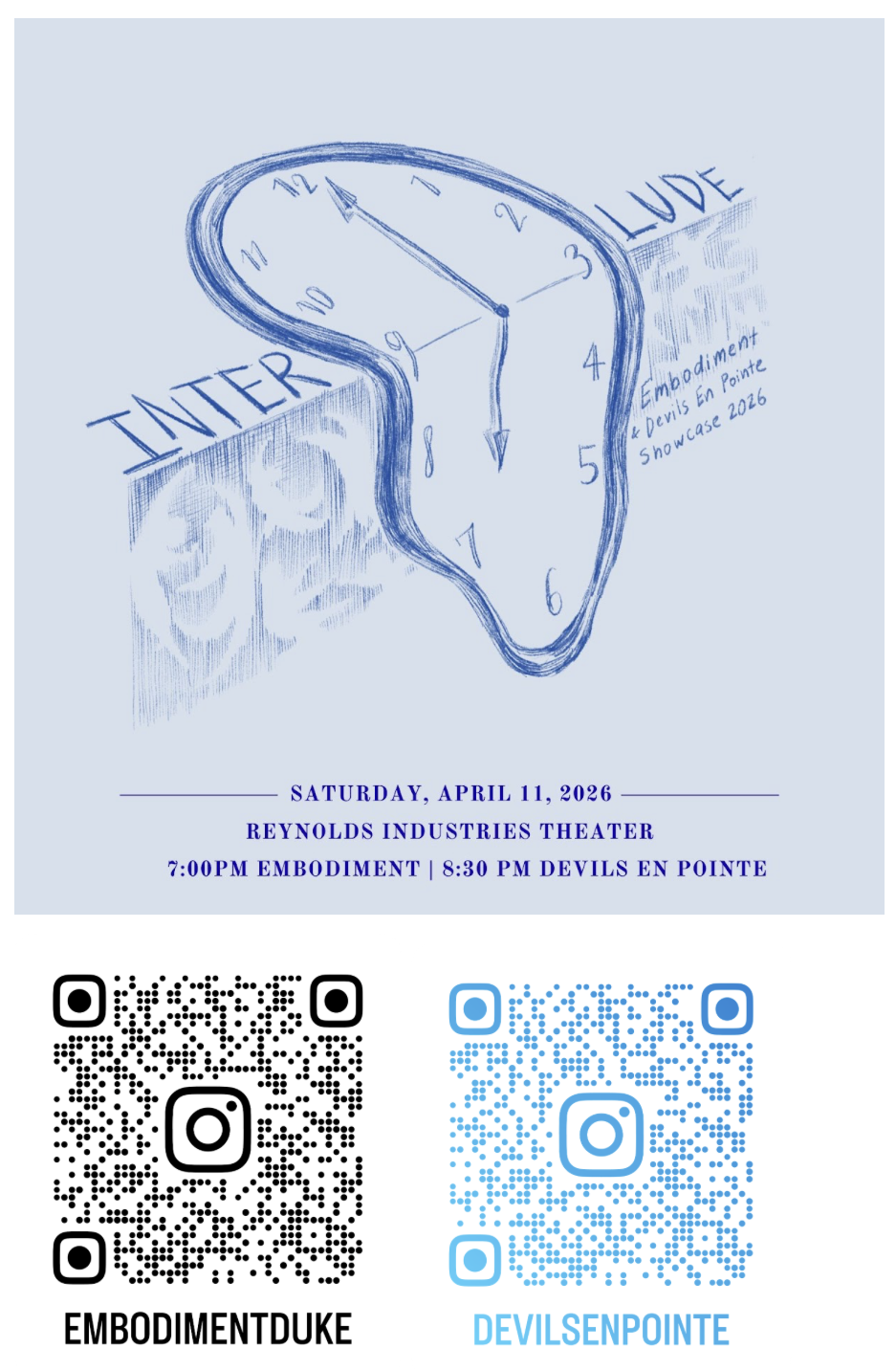
- Devils en Pointe
- Embodiment
- Saturday April 11 @ 7pm
- Reynolds Industries Theater
- Classmates! More Shelly Han!
Saturday: Nakisai Showcase

- Insta: @dukenakisaiade
- Saturday April 11 @ 7pm
- Page Auditorium
- #DOMOREBELIT
Saturday: Pureun Showcase

- Insta: @duke_pureun
- Saturday April 11 @ 8:15pm
- Page Auditorium
- Makky! Mia!
Sunday: Ishq Showcase

- Insta: @duke.ishq
- Sunday April 12 @ 3pm
- Reynolds Theater
- Maaany WANANA alumni
Sunday: Chinese Music Ensemble

- Duke Chinese Music Ensemble
- Sunday April 12 @ 5pm
- Nelson Music Room (East Campus)
- Eric!
Training versus testing data
To mimic this “out-of-sample” idea, we randomly split the data into two parts:
- training data: this is what the model gets to see when we fit it;
- test data: withheld. We assess how well the trained model can predict on this data it hasn’t seen before.

Explore: forested or not
Explore: annual precipitation
Probability to log-odds
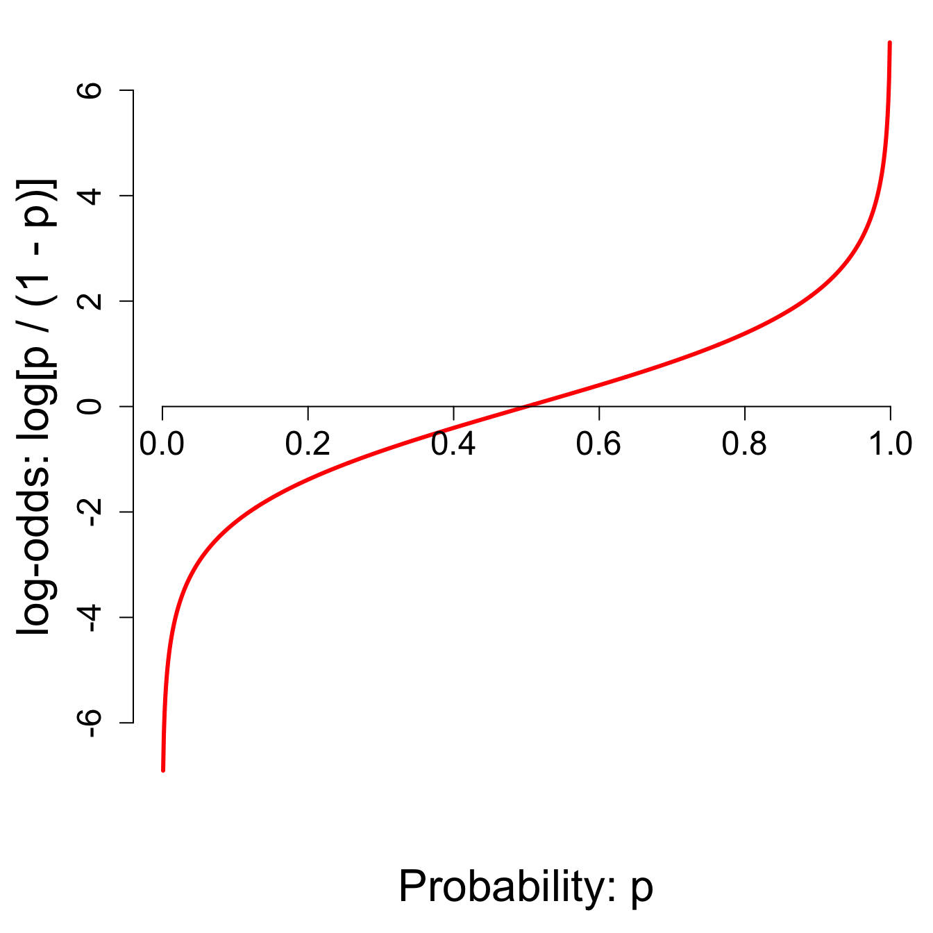
- \(p = 0 \to \text{log-odds}=-\infty\);
- \(p = 1/2 \to \text{log-odds}=0\);
- \(p = 1 \to \text{log-odds}=\infty\);
- And everything in between.
The log-odds transformation takes probabilities between 0 and 1 and streeetches them out to numbers between \(-\infty\) and \(\infty\), for which the linear model is appropriate.
How did the model perform?
These are the four possibilities:
- Our test data have the truth in the
forestedcolumn; - We can compare the predictions in
.pred_classto the true values and see how we did.
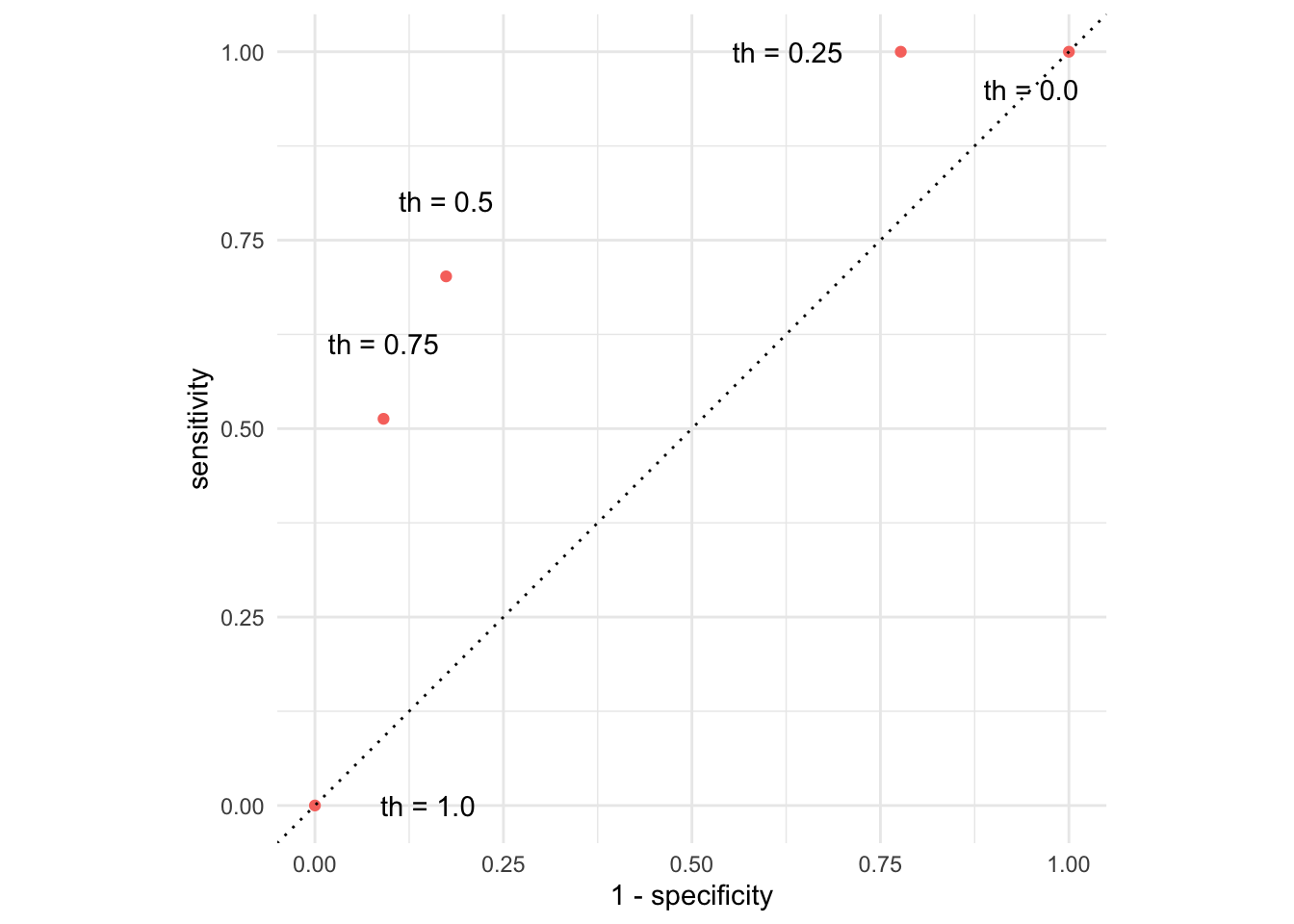
Picture how errors change with threshold (th)
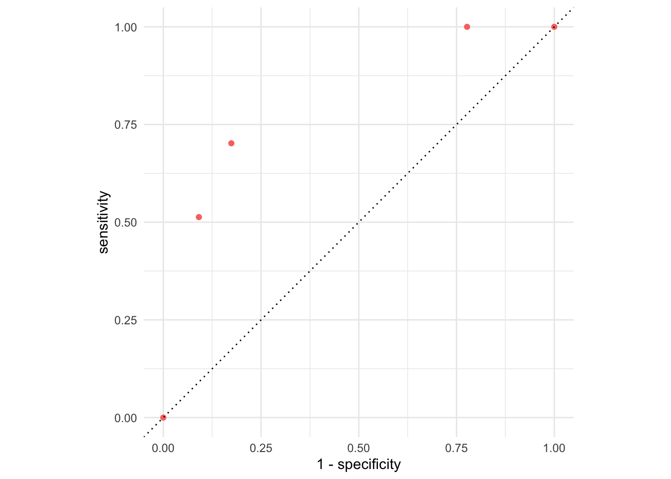
Picture how errors change with threshold (th)
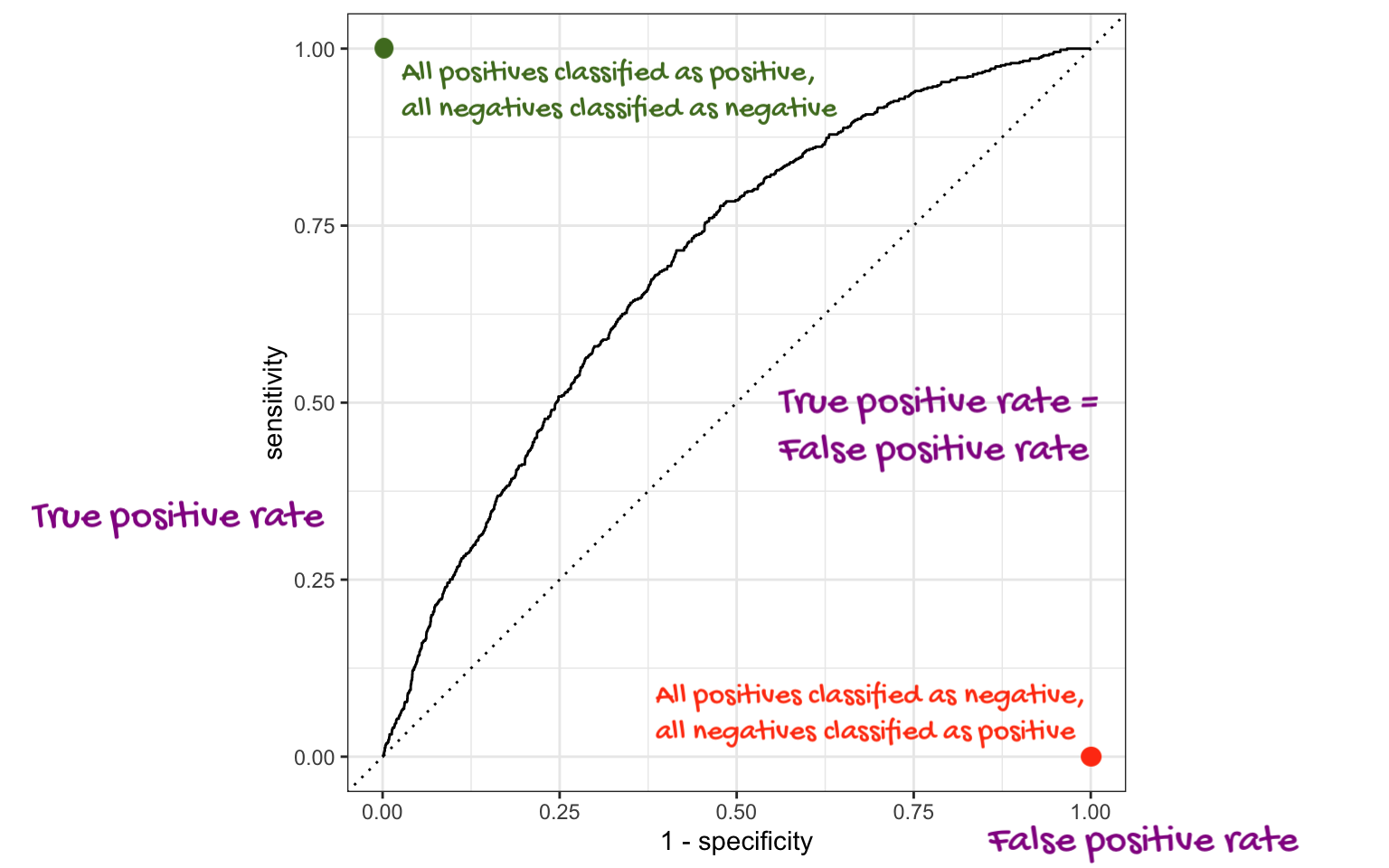
The ROC curve
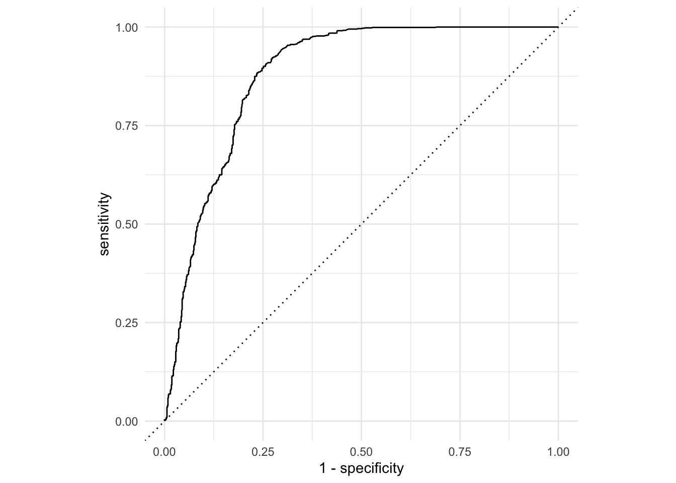
The ROC curve
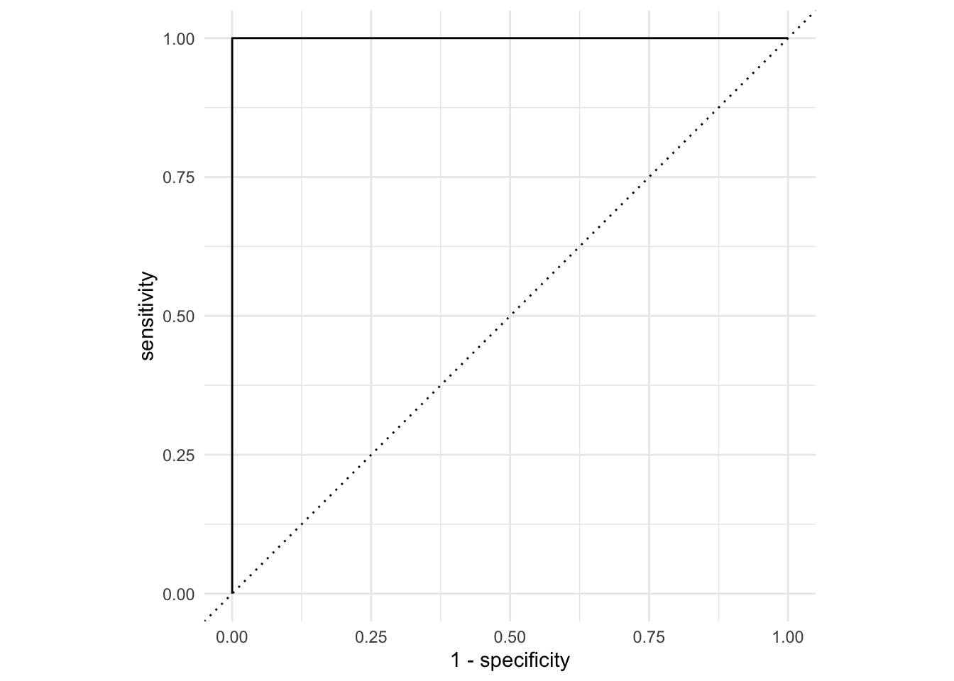
AUC = 1
This is the best we could possibly do:
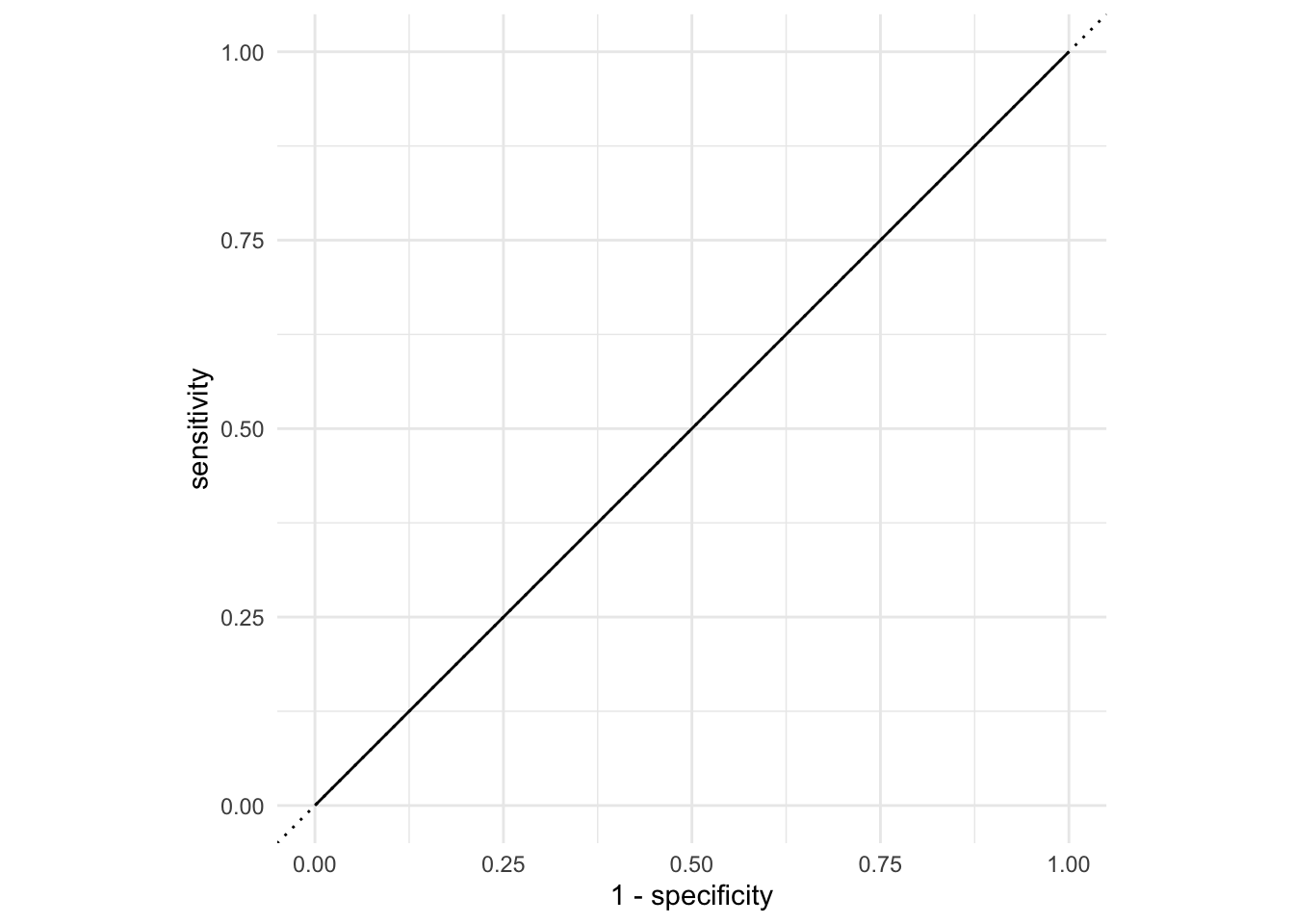
AUC = 1 / 2
Don’t waste time fitting a model. Just flip a coin:
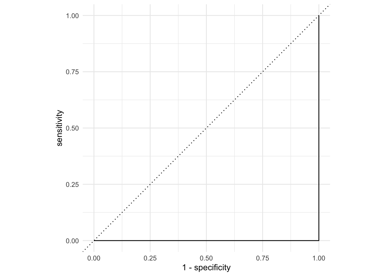
AUC = 0
This is the worst we could possibly do:
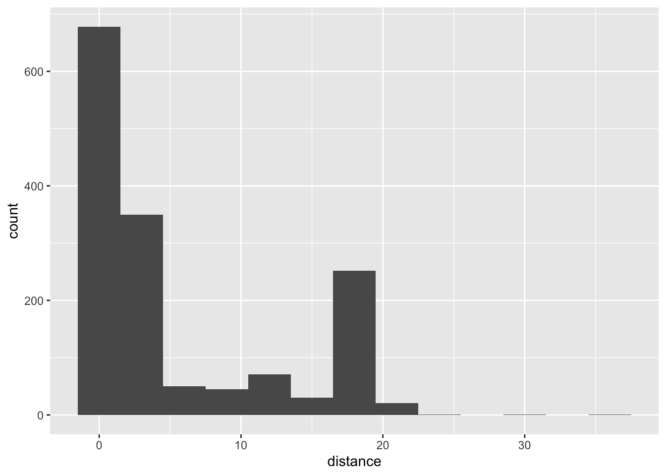
distance
What’s the distribution of distance?
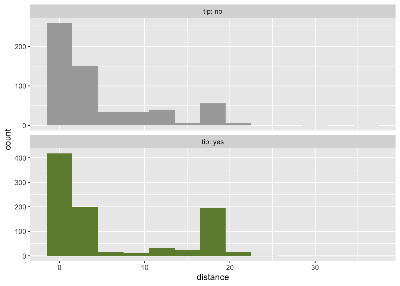
tip and distance
tip and hour
ggplot(chicago_taxi_train, aes(x = hour, fill = tip, group = tip)) +
  geom_histogram(binwidth = 1, show.legend = FALSE) +
  scale_fill_manual(values = c("yes" = "darkolivegreen4", "no" = "darkgray")) +
  scale_x_continuous(breaks = seq(0, 18, by = 6)) +
  facet_wrap(~tip, ncol = 1, labeller = label_both, scales = "free_y")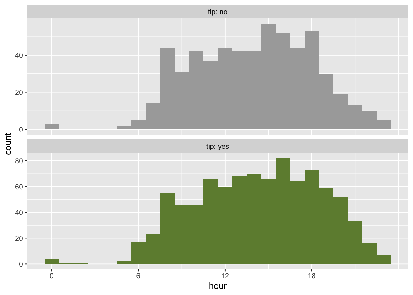
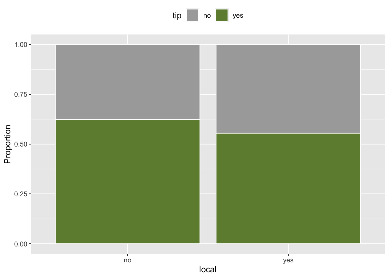
tip and local
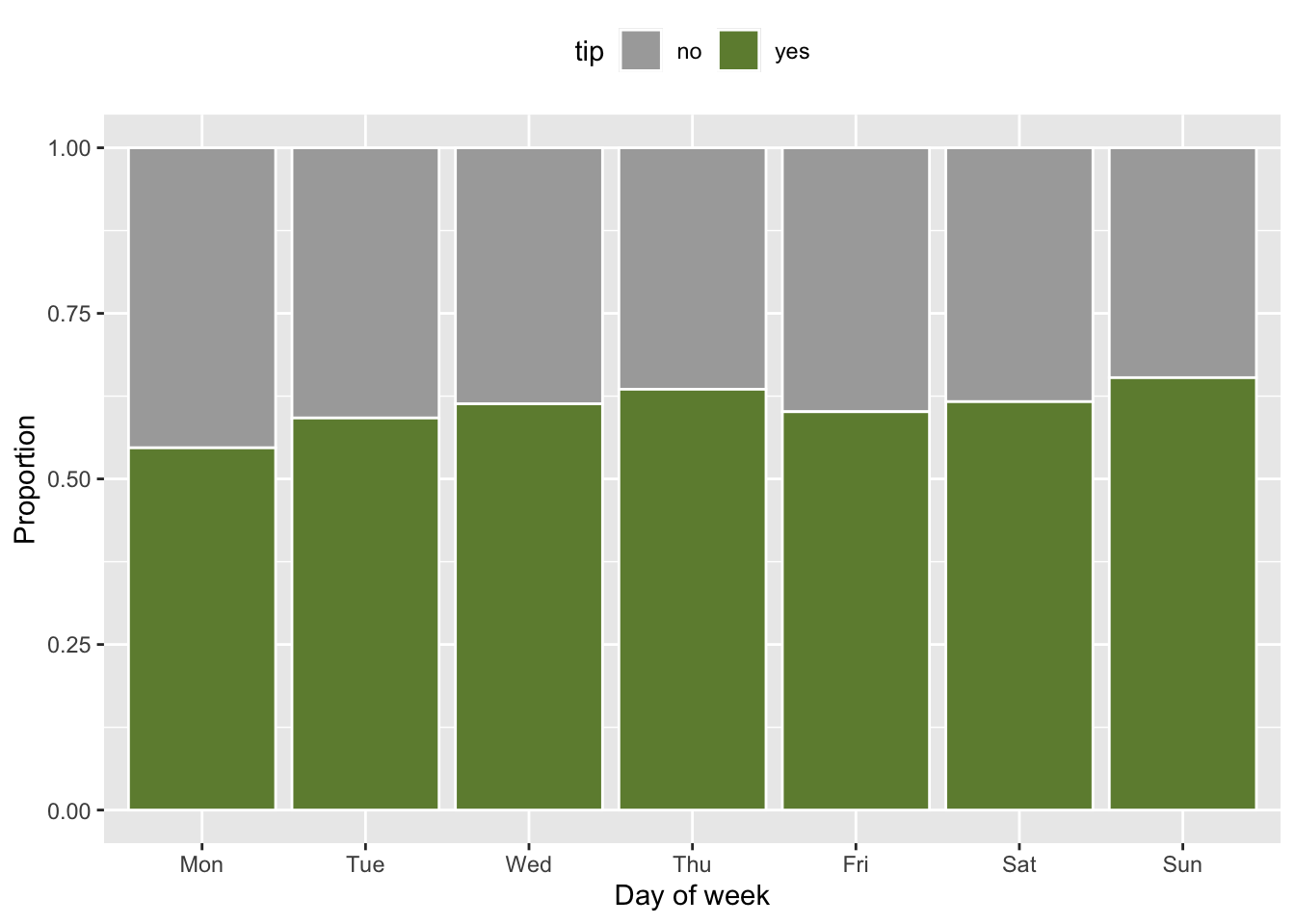
tip and dow