Hypothesis testing

Lecture 23

Author
Affiliation

Josh Lim

Duke University
STA 199 Spring 2026

Published

April 15, 2026

While you wait: Participate 📱💻

Sampling uncertainty refers to…

  • uncertainty about the accuracy of data collection
  • uncertainty about whether our statistical model is true
  • sensitivity of results to human error
  • variation in conclusions across different models
  • variation in estimates across alternative datasets

Scan the QR code or go HERE. Log in with your Duke NetID.

This ain’t Zito

Hi, I’m Josh!

  • 2nd Year PhD Student in Statistical Science
  • Teaching this course in summer
  • Fun fact: I’m a professional Saja Boy (Kpop Demon Hunters)

Zito the GOAT

Hypothesis testing

Hypothesis testing

A hypothesis test is a statistical technique used to evaluate competing claims using data

  • Null hypothesis, \(H_0\): An assumption about the population. “There is nothing going on.”

  • Alternative hypothesis, \(H_A\): A research question about the population. “There is something going on”.

. . .

Note: Hypotheses are always at the population level!

Running Example

glimpse(volleyball)
Rows: 25
Columns: 4
$ name   <chr> "Maguilaura Frias", "Maria Elena Aguilera", "Mitzy Natalia Gonz…
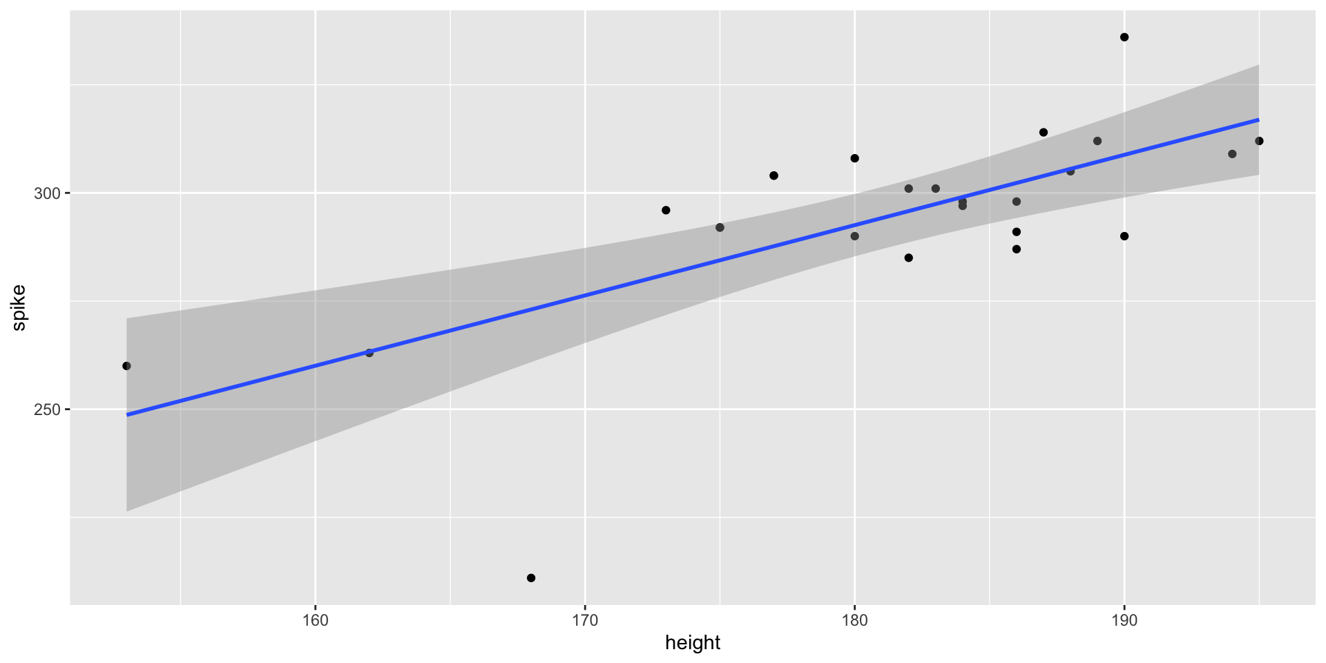
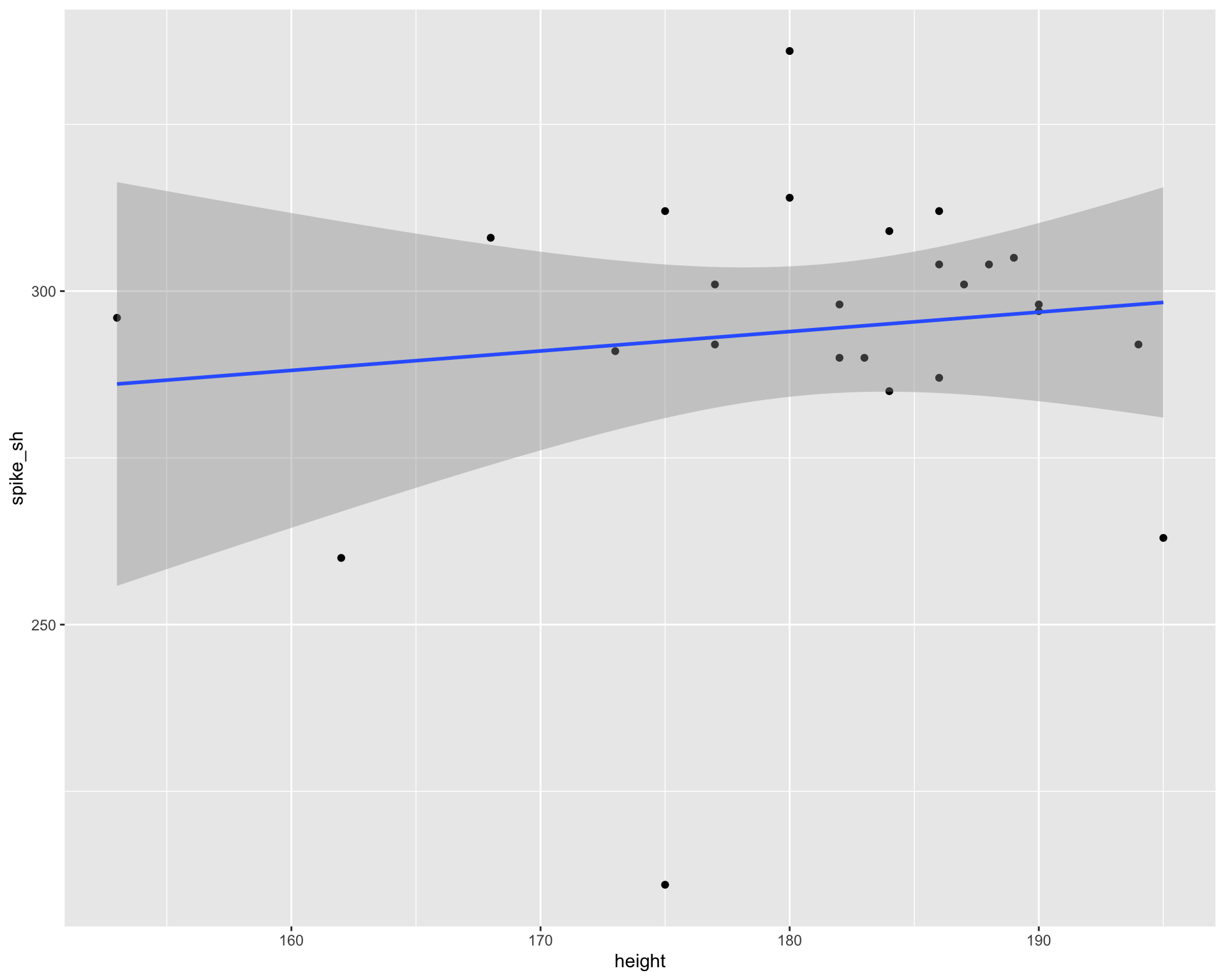
$ height <dbl> 186, 153, 168, 173, 162, 190, 180, 184, 188, 195, 186, 175, 183…
$ spike  <dbl> 291, 260, 211, 296, 263, 290, 308, 298, 305, 312, 298, 292, 301…
$ block  <dbl> 280, 240, 209, 286, 253, 285, 231, 295, 295, 300, 285, 281, 288…
  • Volleyball Dataset on FIVB Athletes
  • Spike: How high an athlete touches on a spike (cm)
  • Block: How high an athlete touches on a block (cm)
  • Height (cm)

Running Example cont

Question: Is an athlete’s spike touch significantly related to their height?

observed_fit <- volleyball |>
  specify(spike ~ height) |>
  fit()

observed_fit
# A tibble: 2 × 2
  term      estimate
  <chr>        <dbl>
1 intercept   0.0540
2 height      1.62  

Setting hypotheses

  • Null hypothesis, \(H_0\): “There is nothing going on.” The slope of the model for predicting the spike touch of FIVB athletes from their heights is 0, \(\beta_1 = 0\).

  • Alternative hypothesis, \(H_A\): “There is something going on”. The slope of the model for predicting the spike touch of FIVB athletes from their heights is different than, \(\beta_1 \ne 0\).

Hypothesis testing “mindset”

  • Assume you live in a world where null hypothesis is true: \(\beta_1 = 0\).

  • Ask yourself how likely you are to observe the sample statistic, or something even more extreme, in this world: \(P(b_1 \leq -1.62~or~b_1 \geq 1.62 | \beta_1 = 0)\) = ?

Hypothesis testing as a court trial

  • Null hypothesis, \(H_0\): Defendant is innocent

  • Alternative hypothesis, \(H_A\): Defendant is guilty

. . .

  • Present the evidence: Collect data

. . .

  • Judge the evidence: “Could these data plausibly have happened by chance if the null hypothesis were true?”
    • Yes: Fail to reject \(H_0\)
    • No: Reject \(H_0\)

Hypothesis testing as medical diagnosis

  • Null hypothesis, \(H_0\): patient is fine

  • Alternative hypothesis, \(H_A\): patient is sick

. . .

  • Present the evidence: Collect data

. . .

  • Judge the evidence: “Could these data plausibly have happened by chance if the null hypothesis were true?”
    • Yes: Fail to reject \(H_0\)
    • No: Reject \(H_0\)

Hypothesis testing framework

  • Start with a null hypothesis, \(H_0\), that represents the status quo

  • Set an alternative hypothesis, \(H_A\), that represents the research question, i.e. what we’re testing for

  • Conduct a hypothesis test under the assumption that the null hypothesis is true and calculate a p-value (probability of observed or more extreme outcome given that the null hypothesis is true)

    • if the test results suggest that the data do not provide convincing evidence for the alternative hypothesis, stick with the null hypothesis
    • if they do, then reject the null hypothesis in favor of the alternative

Calculate observed slope

… which we have already done:

observed_fit <- volleyball |>
  specify(spike ~ height) |>
  fit()

observed_fit
# A tibble: 2 × 2
  term      estimate
  <chr>        <dbl>
1 intercept   0.0540
2 height      1.62  

Simulate null distribution

set.seed(24601)
null_dist <- volleyball |>
  specify(spike ~ height) |>
  hypothesize(null = "independence") |>
  generate(reps = 10000, type = "permute") |>
  fit()

Wait, so what’s a null distribution?

  • Simulating a universe under \(H_0\): the slope of the model for predicting the spike touch of FIVB athletes from their heights is 0, \(\beta_1 = 0\). I.e., no relationship between spike and height.

  • If I “shuffle” the order of the spike variable, is there a relationship between spike and height? Could height predict spike touch?

Participate 📱💻

If I “shuffle” the order of the spike variable, is there a relationship between spike and height? Could height predict spike touch?

  • On Average, Yes
  • On Average, No
  • Never
  • I want lunch, stop talking about volleyball

Scan the QR code or go HERE. Log in with your Duke NetID.

Shuffling is cool, trust

  • On avergage, no

  • Shuffling breaks any link between spike and height (on average)

  • type = "permute"

  • Shuffle the spike variable, fit a model and get a slope, record the slope, repeat!

  • If the null is true, the distribution of these slopes should be centered on zero!

  • More on this in STA 221L

  • What if we shuffled height instead? Both?

Every day I’m shuffling

ggplot(volleyball, aes(x = height, y = spike)) +
  geom_point() + 
  geom_smooth(method = "lm")

Every day I’m shuffling

ggplot(volleyball, aes(x = height, y = sample(spike))) +
  geom_point() + 
  geom_smooth(method = "lm")

Wait, what’s that new function

rouges_gallery <- c("Josh Lim", "John Zito", "Sarah Wu", "Katie Solarz")
rouges_gallery
[1] "Josh Lim"     "John Zito"    "Sarah Wu"     "Katie Solarz"

. . .

set.seed(8675309)

sample(rouges_gallery)
[1] "Katie Solarz" "Sarah Wu"     "John Zito"    "Josh Lim"    

What if this was my shuffle?

# A tibble: 2 × 2
  term        estimate
  <chr>          <dbl>
1 (Intercept)  336.   
2 height        -0.231

What if this was my shuffle instead?

# A tibble: 2 × 2
  term        estimate
  <chr>          <dbl>
1 (Intercept)  389.   
2 height        -0.526

What if this was my shuffle instead?

# A tibble: 2 × 2
  term        estimate
  <chr>          <dbl>
1 (Intercept)  242.   
2 height         0.291

Rinse and repeat 10000 times…

View null distribution

null_dist
# A tibble: 20,000 × 3
# Groups:   replicate [10,000]
   replicate term      estimate
       <int> <chr>        <dbl>
 1         1 intercept 292.    
 2         1 height      0.0132
 3         2 intercept 301.    
 4         2 height     -0.0377
 5         3 intercept 402.    
 6         3 height     -0.594 
 7         4 intercept 366.    
 8         4 height     -0.395 
 9         5 intercept 449.    
10         5 height     -0.853 
# ℹ 19,990 more rows

Visualize null distribution

null_dist |>
  filter(term == "height") |>
  ggplot(aes(x = estimate)) +
  geom_histogram(binwidth = 0.2)

Reminder: observed fit

What was our estimate to begin with?

observed_fit <- volleyball |>
  specify(spike ~ height) |>
  fit()

observed_fit
# A tibble: 2 × 2
  term      estimate
  <chr>        <dbl>
1 intercept   0.0540
2 height      1.62  

Visualize null distribution (alternative)

visualize(null_dist) +
  shade_p_value(obs_stat = observed_fit, direction = "two-sided")

Get p-value

null_dist |>
  get_p_value(obs_stat = observed_fit, direction = "two-sided")
# A tibble: 2 × 2
  term      p_value
  <chr>       <dbl>
1 height      0.002
2 intercept   0.002

Make a decision

Based on the p-value calculated, what is the conclusion of the hypothesis test?

  • Probability of observing your data or something more extreme given the null is true
  • Since \(p = 0.002\), we reject the null hypothesis and have evidence that there is a statistically significant relationship between an FIVB players spike touch and height.

How small is small enough?

Pick a threshold \(\alpha\in[0,\,1]\) called the discernibility level and threshold the \(p\)-value:

  • If \(p\text{-value} < \alpha\), reject null and accept alternative;
  • If \(p\text{-value} \geq \alpha\), fail to reject null;

Sometimes the test will be wrong

Think about the judge

\(H_0\) person innocent vs \(H_A\) person guilty

Think about the doctor

\(H_0\) person well vs \(H_A\) person sick.

Where does alpha come in to this?