Exploring data I
Lecture 4
While you wait…
Prepare for today’s application exercise: ae-04-gerrymander-explore-I
Switch to your
aeproject in RStudio;Make sure all of your changes up to this point are committed (ie there’s nothing left in your Git pane);
Click Pull to get today’s application exercise file: ae-04-gerrymander-explore-I.qmd.
Then push. So Render > Commit > Pull > Push.
(To see the new file, you may have to refresh the Files pane by clicking “Home”)
Wait till the you’re prompted to work on the application exercise during class before editing the file.
Exploratory data analysis
So far…
| Data set | Occasion | Source | A row was a… |
|---|---|---|---|
age_guesses |
Lecture 0 | file | STAAWANANA student |
penguins |
Lecture 1 | package | penguin |
unvotes |
Lecture 2 | package | year-issue-country |
nc_county |
Lab, HW | file | NC county |
bechdel |
Lecture 3 | file | film |
gerrymander |
Lecture 4 | package | district |
Packages
- For the data: usdata
── Attaching core tidyverse packages ──────────────────────── tidyverse 2.0.0 ──
✔ dplyr     1.1.4     ✔ readr     2.1.5
✔ forcats   1.0.0     ✔ stringr   1.5.1
✔ ggplot2   4.0.2     ✔ tibble    3.3.0
✔ lubridate 1.9.4     ✔ tidyr     1.3.1
✔ purrr     1.1.0
── Conflicts ────────────────────────────────────────── tidyverse_conflicts() ──
✖ dplyr::filter() masks stats::filter()
✖ dplyr::lag()    masks stats::lag()
ℹ Use the conflicted package (<http://conflicted.r-lib.org/>) to force all conflicts to become errorsData: gerrymander
gerrymander# A tibble: 435 × 12
district last_name first_name party16 clinton16 trump16 dem16 state party18
<chr> <chr> <chr> <chr> <dbl> <dbl> <dbl> <chr> <chr>
1 AK-AL Young Don R 37.6 52.8 0 AK R
2 AL-01 Byrne Bradley R 34.1 63.5 0 AL R
3 AL-02 Roby Martha R 33 64.9 0 AL R
4 AL-03 Rogers Mike D. R 32.3 65.3 0 AL R
5 AL-04 Aderholt Rob R 17.4 80.4 0 AL R
6 AL-05 Brooks Mo R 31.3 64.7 0 AL R
7 AL-06 Palmer Gary R 26.1 70.8 0 AL R
8 AL-07 Sewell Terri D 69.8 28.6 1 AL D
9 AR-01 Crawford Rick R 30.2 65 0 AR R
10 AR-02 Hill French R 41.7 52.4 0 AR R
# ℹ 425 more rows
# ℹ 3 more variables: dem18 <dbl>, flip18 <dbl>, gerry <fct>What is gerrymandering?
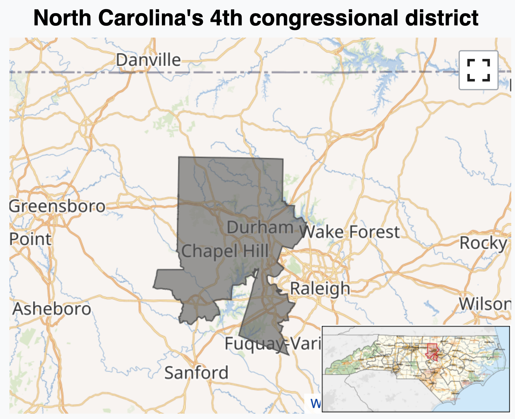
JZ’s tour of the USA
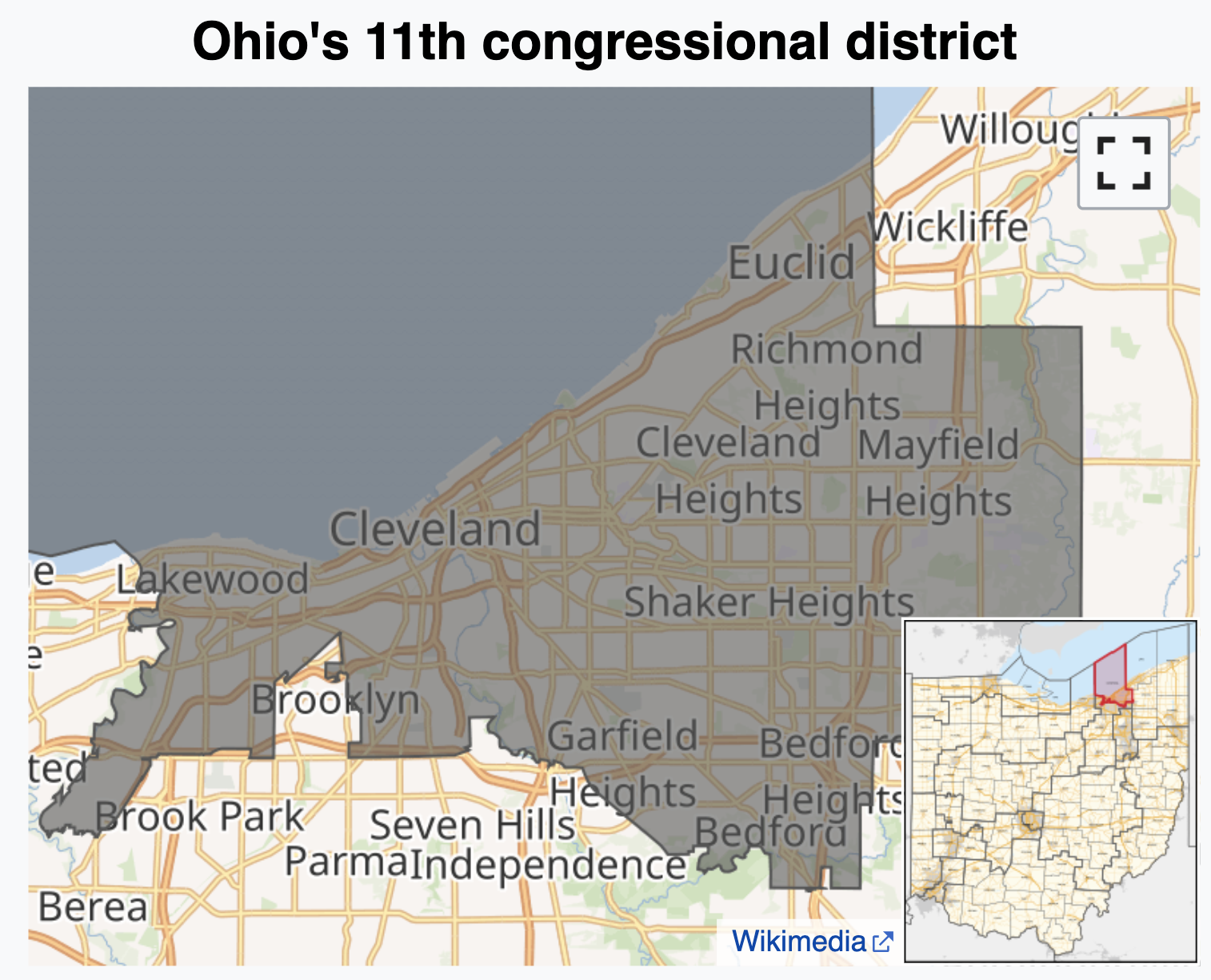
JZ’s tour of the USA
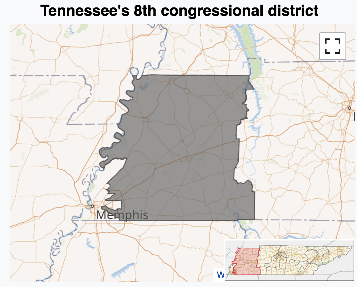
JZ’s tour of the USA
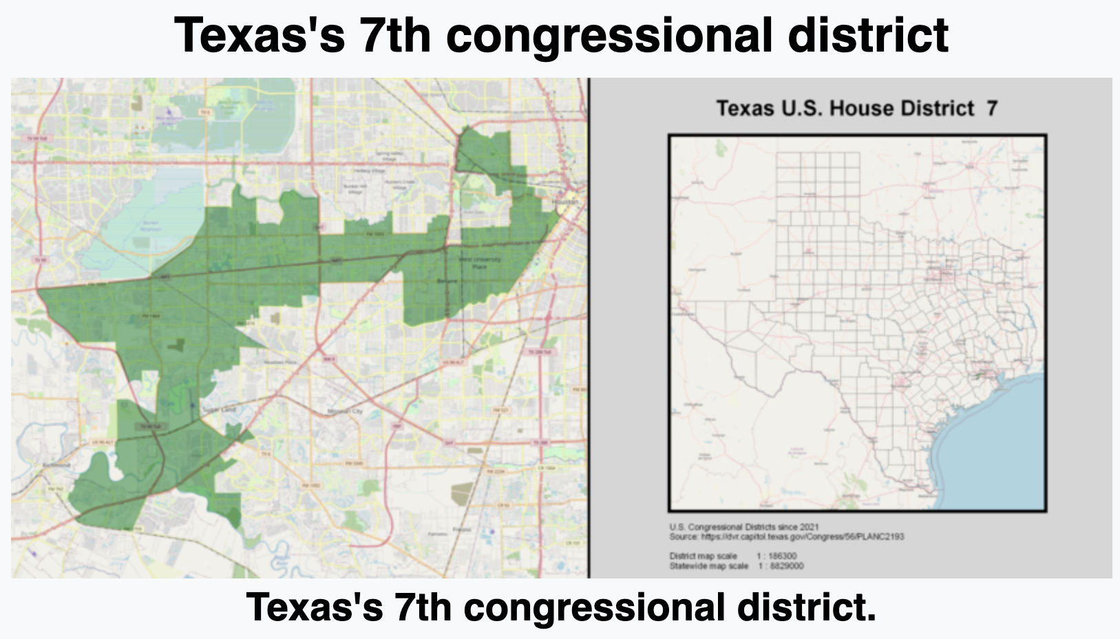
JZ’s tour of the USA
Data: gerrymander
What is a good first function to use to get to know a dataset?
glimpse(gerrymander)Rows: 435
Columns: 12
$ district <chr> "AK-AL", "AL-01", "AL-02", "AL-03", "AL-04", "AL-05", "AL-0…
$ last_name <chr> "Young", "Byrne", "Roby", "Rogers", "Aderholt", "Brooks", "…
$ first_name <chr> "Don", "Bradley", "Martha", "Mike D.", "Rob", "Mo", "Gary",…
$ party16 <chr> "R", "R", "R", "R", "R", "R", "R", "D", "R", "R", "R", "R",…
$ clinton16 <dbl> 37.6, 34.1, 33.0, 32.3, 17.4, 31.3, 26.1, 69.8, 30.2, 41.7,…
$ trump16 <dbl> 52.8, 63.5, 64.9, 65.3, 80.4, 64.7, 70.8, 28.6, 65.0, 52.4,…
$ dem16 <dbl> 0, 0, 0, 0, 0, 0, 0, 1, 0, 0, 0, 0, 1, 0, 1, 0, 0, 0, 1, 0,…
$ state <chr> "AK", "AL", "AL", "AL", "AL", "AL", "AL", "AL", "AR", "AR",…
$ party18 <chr> "R", "R", "R", "R", "R", "R", "R", "D", "R", "R", "R", "R",…
$ dem18 <dbl> 0, 0, 0, 0, 0, 0, 0, 1, 0, 0, 0, 0, 1, 1, 1, 0, 0, 0, 1, 0,…
$ flip18 <dbl> 0, 0, 0, 0, 0, 0, 0, 0, 0, 0, 0, 0, 0, 1, 0, 0, 0, 0, 0, 0,…
$ gerry <fct> mid, high, high, high, high, high, high, high, mid, mid, mi…Data: gerrymander
Rows: Congressional districts
-
Columns:
Congressional district and state
2016 election: winning party, % for Clinton, % for Trump, whether a Democrat won the House election, name of election winner
2018 election: winning party, whether a Democrat won the 2018 House election
Whether a Democrat flipped the seat in the 2018 election
Prevalence of gerrymandering: low, mid, and high
Variable types: district
| Variable | Type |
|---|---|
district |
categorical, ID |
last_name |
|
first_name |
|
party16 |
|
clinton16 |
|
trump16 |
|
dem16 |
|
state |
|
party18 |
|
dem18 |
|
flip18 |
|
gerry |
Congressional district:
gerrymander |>
  select(district)
# A tibble: 435 × 1
district
<chr>
1 AK-AL
2 AL-01
3 AL-02
4 AL-03
5 AL-04
6 AL-05
7 AL-06
8 AL-07
9 AR-01
10 AR-02
# ℹ 425 more rowsVariable types: last_name
| Variable | Type |
|---|---|
district |
categorical, ID |
last_name |
categorical, ID |
first_name |
|
party16 |
|
clinton16 |
|
trump16 |
|
dem16 |
|
state |
|
party18 |
|
dem18 |
|
flip18 |
|
gerry |
Last name of 2016 election winner:
gerrymander |>
  select(last_name)
# A tibble: 435 × 1
last_name
<chr>
1 Young
2 Byrne
3 Roby
4 Rogers
5 Aderholt
6 Brooks
7 Palmer
8 Sewell
9 Crawford
10 Hill
# ℹ 425 more rowsVariable types: first_name
| Variable | Type |
|---|---|
district |
categorical, ID |
last_name |
categorical, ID |
first_name |
categorical, ID |
party16 |
|
clinton16 |
|
trump16 |
|
dem16 |
|
state |
|
party18 |
|
dem18 |
|
flip18 |
|
gerry |
First name of 2016 election winner:
gerrymander |>
  select(first_name)
# A tibble: 435 × 1
first_name
<chr>
1 Don
2 Bradley
3 Martha
4 Mike D.
5 Rob
6 Mo
7 Gary
8 Terri
9 Rick
10 French
# ℹ 425 more rowsVariable types: party16
| Variable | Type |
|---|---|
district |
categorical, ID |
last_name |
categorical, ID |
first_name |
categorical, ID |
party16 |
categorical |
clinton16 |
|
trump16 |
|
dem16 |
|
state |
|
party18 |
|
dem18 |
|
flip18 |
|
gerry |
Political party of 2016 election winner:
gerrymander |>
  select(party16)
# A tibble: 435 × 1
party16
<chr>
1 R
2 R
3 R
4 R
5 R
6 R
7 R
8 D
9 R
10 R
# ℹ 425 more rowsVariable types: clinton16
| Variable | Type |
|---|---|
district |
categorical, ID |
last_name |
categorical, ID |
first_name |
categorical, ID |
party16 |
categorical |
clinton16 |
numerical, continuous |
trump16 |
|
dem16 |
|
state |
|
party18 |
|
dem18 |
|
flip18 |
|
gerry |
Percent of vote received by Clinton in 2016 Presidential Election:
gerrymander |>
  select(clinton16)
# A tibble: 435 × 1
clinton16
<dbl>
1 37.6
2 34.1
3 33
4 32.3
5 17.4
6 31.3
7 26.1
8 69.8
9 30.2
10 41.7
# ℹ 425 more rowsVariable types: trump16
| Variable | Type |
|---|---|
district |
categorical, ID |
last_name |
categorical, ID |
first_name |
categorical, ID |
party16 |
categorical |
clinton16 |
numerical, continuous |
trump16 |
numerical, continuous |
dem16 |
|
state |
|
party18 |
|
dem18 |
|
flip18 |
|
gerry |
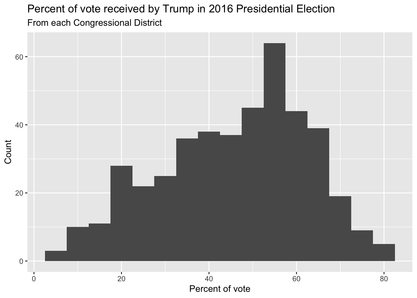
Percent of vote received by Trump in 2016 Presidential Election:
gerrymander |>
  select(trump16)
# A tibble: 435 × 1
trump16
<dbl>
1 52.8
2 63.5
3 64.9
4 65.3
5 80.4
6 64.7
7 70.8
8 28.6
9 65
10 52.4
# ℹ 425 more rowsVariable types: dem16
| Variable | Type |
|---|---|
district |
categorical, ID |
last_name |
categorical, ID |
first_name |
categorical, ID |
party16 |
categorical |
clinton16 |
numerical, continuous |
trump16 |
numerical, continuous |
dem16 |
categorical |
state |
|
party18 |
|
dem18 |
|
flip18 |
|
gerry |
Did a Democrat win the 2016 House election. Levels of 1 (yes) and 0 (no):
gerrymander |>
  select(dem16)
# A tibble: 435 × 1
dem16
<dbl>
1 0
2 0
3 0
4 0
5 0
6 0
7 0
8 1
9 0
10 0
# ℹ 425 more rowsVariable types: state
| Variable | Type |
|---|---|
district |
categorical, ID |
last_name |
categorical, ID |
first_name |
categorical, ID |
party16 |
categorical |
clinton16 |
numerical, continuous |
trump16 |
numerical, continuous |
dem16 |
categorical |
state |
categorical |
party18 |
|
dem18 |
|
flip18 |
|
gerry |
State the Representative is from:
gerrymander |>
  select(state)
# A tibble: 435 × 1
state
<chr>
1 AK
2 AL
3 AL
4 AL
5 AL
6 AL
7 AL
8 AL
9 AR
10 AR
# ℹ 425 more rowsVariable types: party18
| Variable | Type |
|---|---|
district |
categorical, ID |
last_name |
categorical, ID |
first_name |
categorical, ID |
party16 |
categorical |
clinton16 |
numerical, continuous |
trump16 |
numerical, continuous |
dem16 |
categorical |
state |
categorical |
party18 |
categorical |
dem18 |
|
flip18 |
|
gerry |
Political Party of the 2018 election winner:
gerrymander |>
  select(party18)
# A tibble: 435 × 1
party18
<chr>
1 R
2 R
3 R
4 R
5 R
6 R
7 R
8 D
9 R
10 R
# ℹ 425 more rowsVariable types: dem18
| Variable | Type |
|---|---|
district |
categorical, ID |
last_name |
categorical, ID |
first_name |
categorical, ID |
party16 |
categorical |
clinton16 |
numerical, continuous |
trump16 |
numerical, continuous |
dem16 |
categorical |
state |
categorical |
party18 |
categorical |
dem18 |
categorical |
flip18 |
|
gerry |
Did a Democrat win the 2018 House election. Levels of 1 (yes) and 0 (no):
gerrymander |>
  select(dem18)
# A tibble: 435 × 1
dem18
<dbl>
1 0
2 0
3 0
4 0
5 0
6 0
7 0
8 1
9 0
10 0
# ℹ 425 more rowsVariable types: flip18
| Variable | Type |
|---|---|
district |
categorical, ID |
last_name |
categorical, ID |
first_name |
categorical, ID |
party16 |
categorical |
clinton16 |
numerical, continuous |
trump16 |
numerical, continuous |
dem16 |
categorical |
state |
categorical |
party18 |
categorical |
dem18 |
categorical |
flip18 |
categorical |
gerry |
In the 2018 election, did the seat flip from D to R (-1), from R to D (1), or not change (0)?
gerrymander |>
  select(flip18)
# A tibble: 435 × 1
flip18
<dbl>
1 0
2 0
3 0
4 0
5 0
6 0
7 0
8 0
9 0
10 0
# ℹ 425 more rowsVariable types: gerry
| Variable | Type |
|---|---|
district |
categorical, ID |
last_name |
categorical, ID |
first_name |
categorical, ID |
party16 |
categorical |
clinton16 |
numerical, continuous |
trump16 |
numerical, continuous |
dem16 |
categorical |
state |
categorical |
party18 |
categorical |
dem18 |
categorical |
flip18 |
categorical |
gerry |
categorical, ordinal |
Categorical variable for prevalence of gerrymandering with levels of low, mid and high:
gerrymander |>
  select(gerry)
# A tibble: 435 × 1
gerry
<fct>
1 mid
2 high
3 high
4 high
5 high
6 high
7 high
8 high
9 mid
10 mid
# ℹ 425 more rowsUnivariate analysis
Univariate analysis
Analyzing a single variable:
Numerical: histogram, box plot, density plot, etc.
Categorical: bar plot, pie chart, etc.
Histogram - Step 1
ggplot(gerrymander)
Histogram - Step 2

Histogram - Step 3
Histogram - Step 4
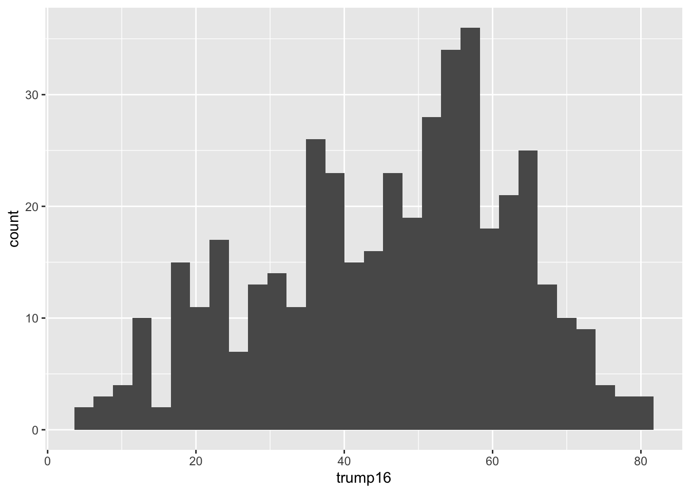
ggplot(gerrymander, aes(x = trump16)) +
  geom_histogram(binwidth = 1)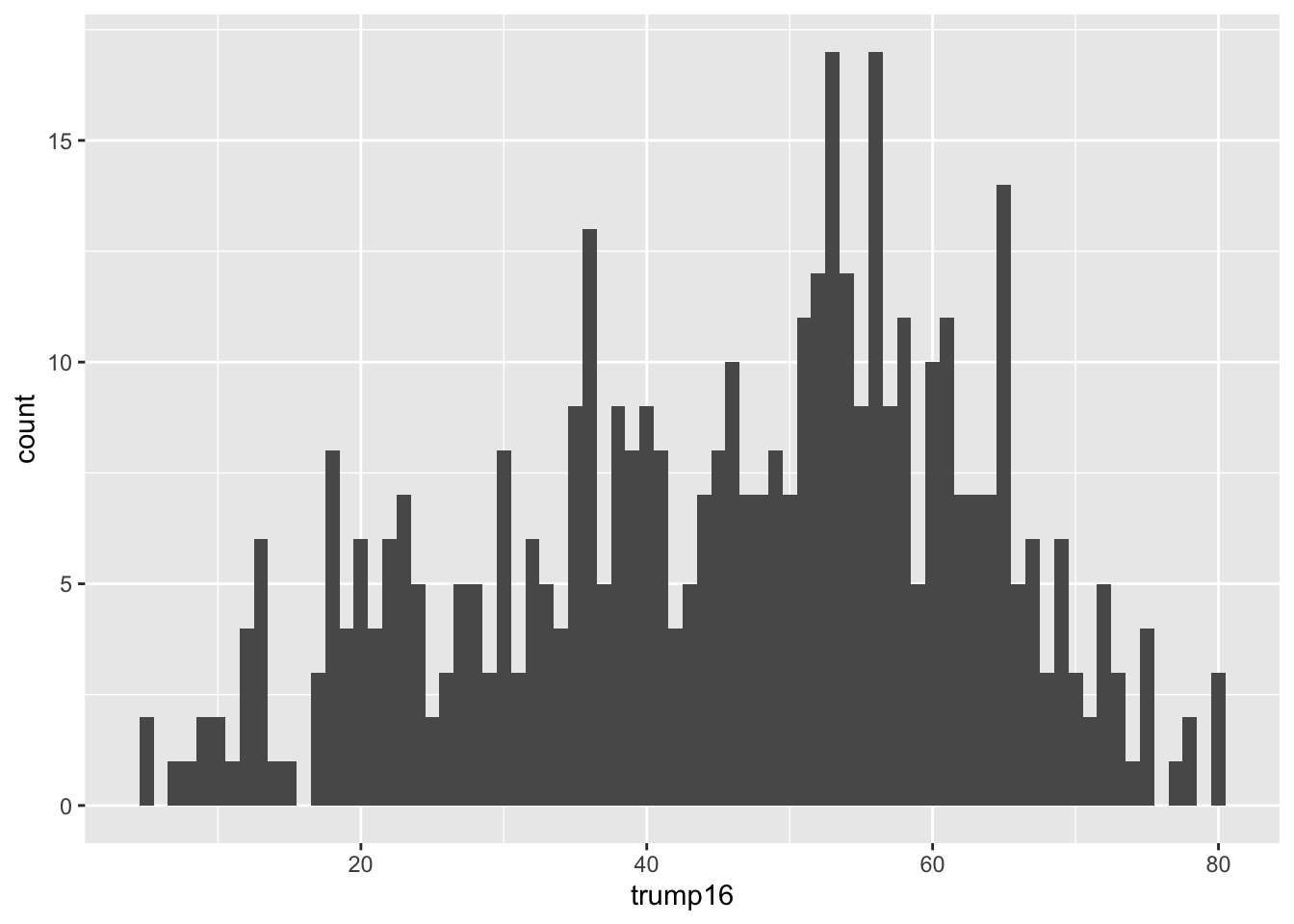
Histogram - Step 4
ggplot(gerrymander, aes(x = trump16)) +
  geom_histogram(binwidth = 100)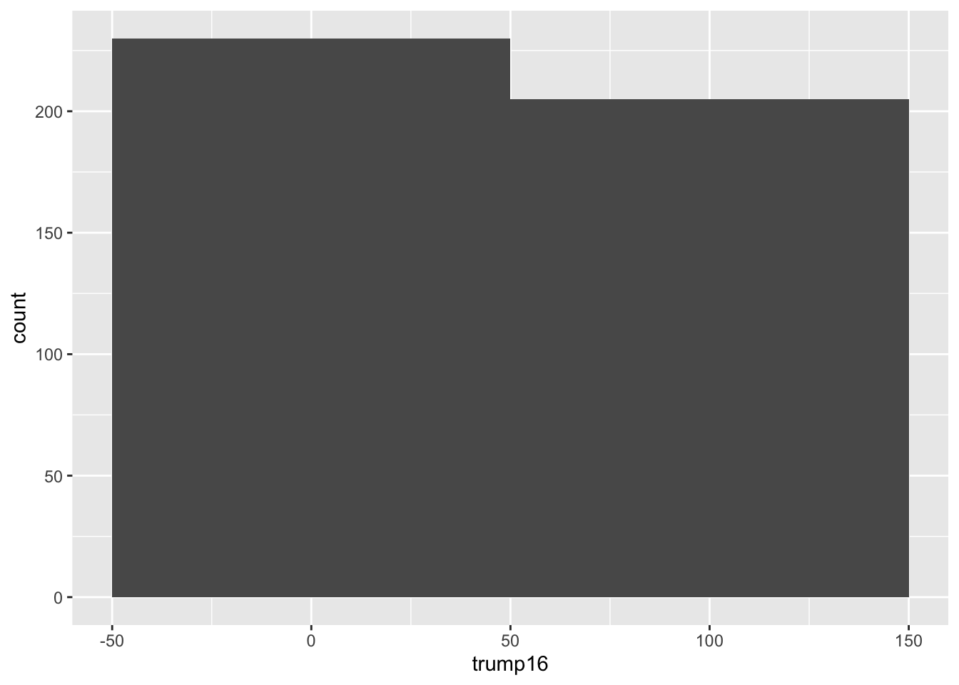
Histogram - Step 4
ggplot(gerrymander, aes(x = trump16)) +
  geom_histogram(binwidth = 3)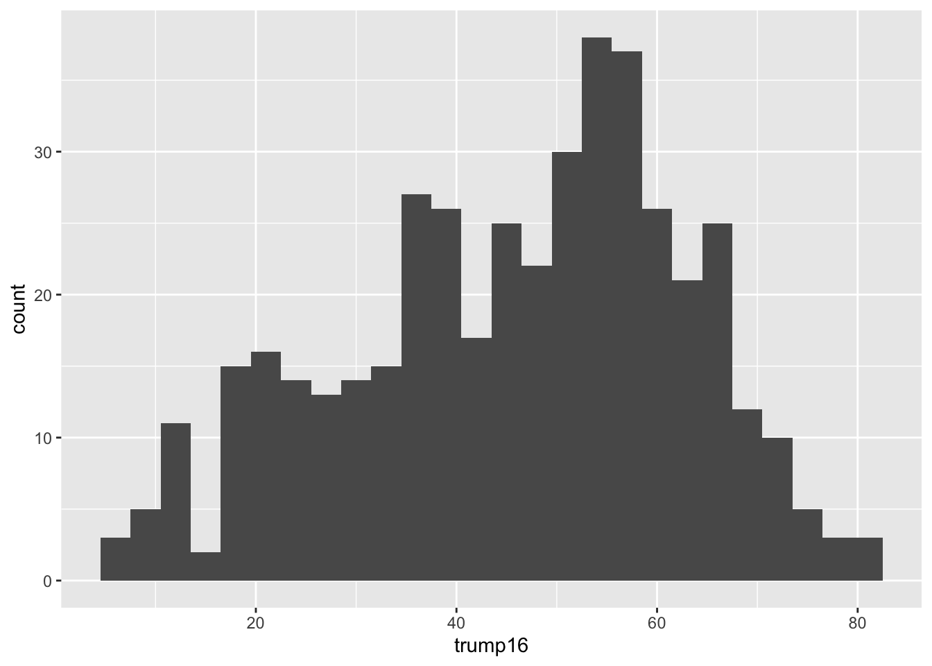
Histogram - Step 4
ggplot(gerrymander, aes(x = trump16)) +
  geom_histogram(binwidth = 5)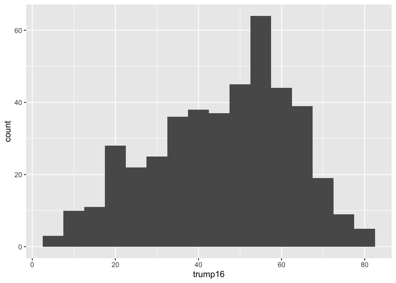
Histogram - Step 5
Box plot - Step 1
ggplot(gerrymander)
Box plot - Step 2
Box plot - Step 3
Box plot - Alternative Step 2 + 3
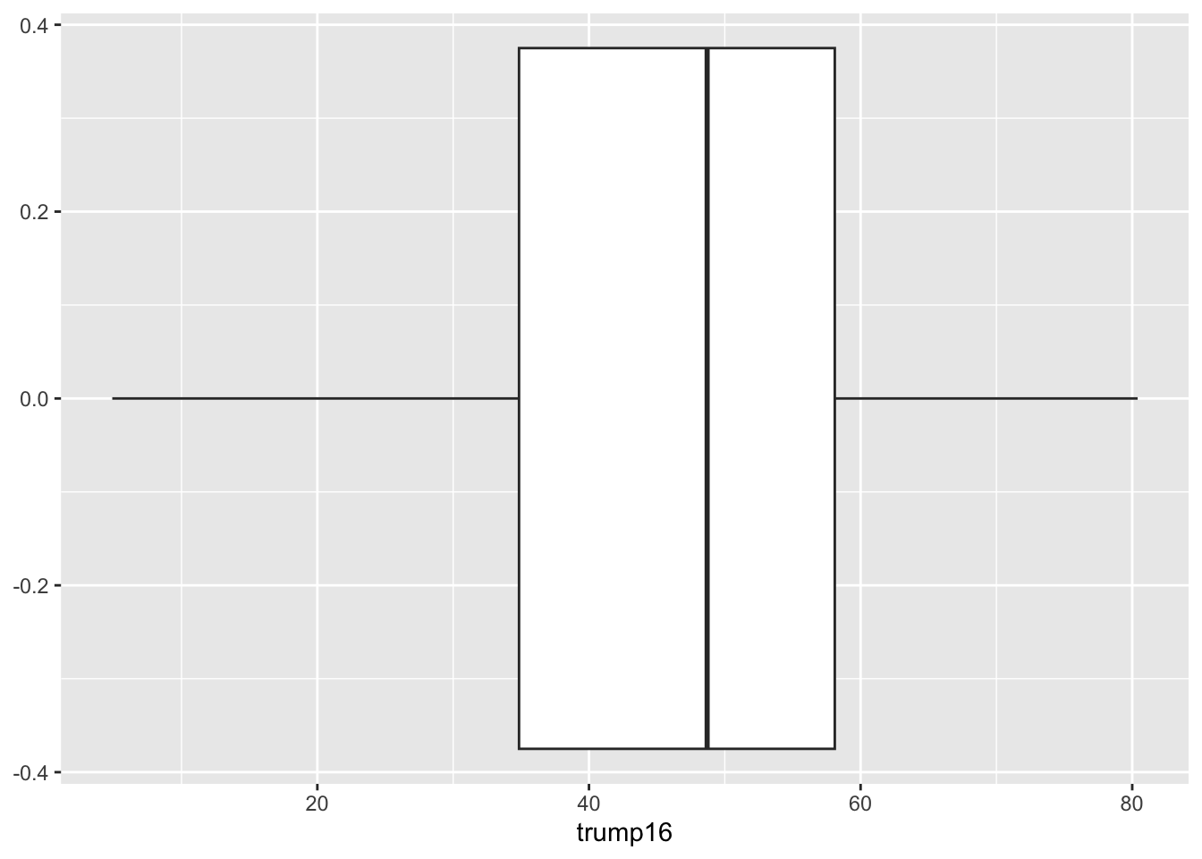
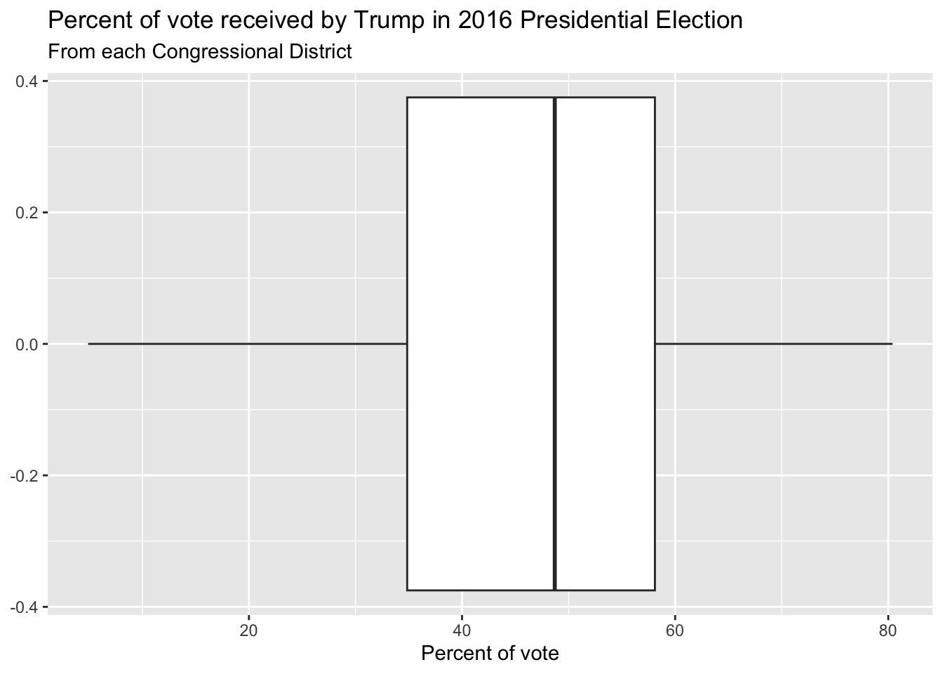
ggplot(gerrymander, aes(y = trump16)) +
  geom_boxplot()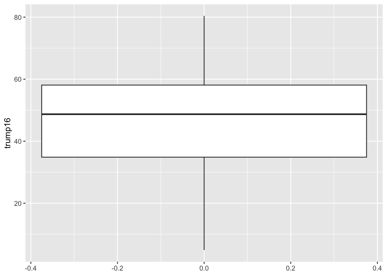
Box plot - Step 4
Whence the box?
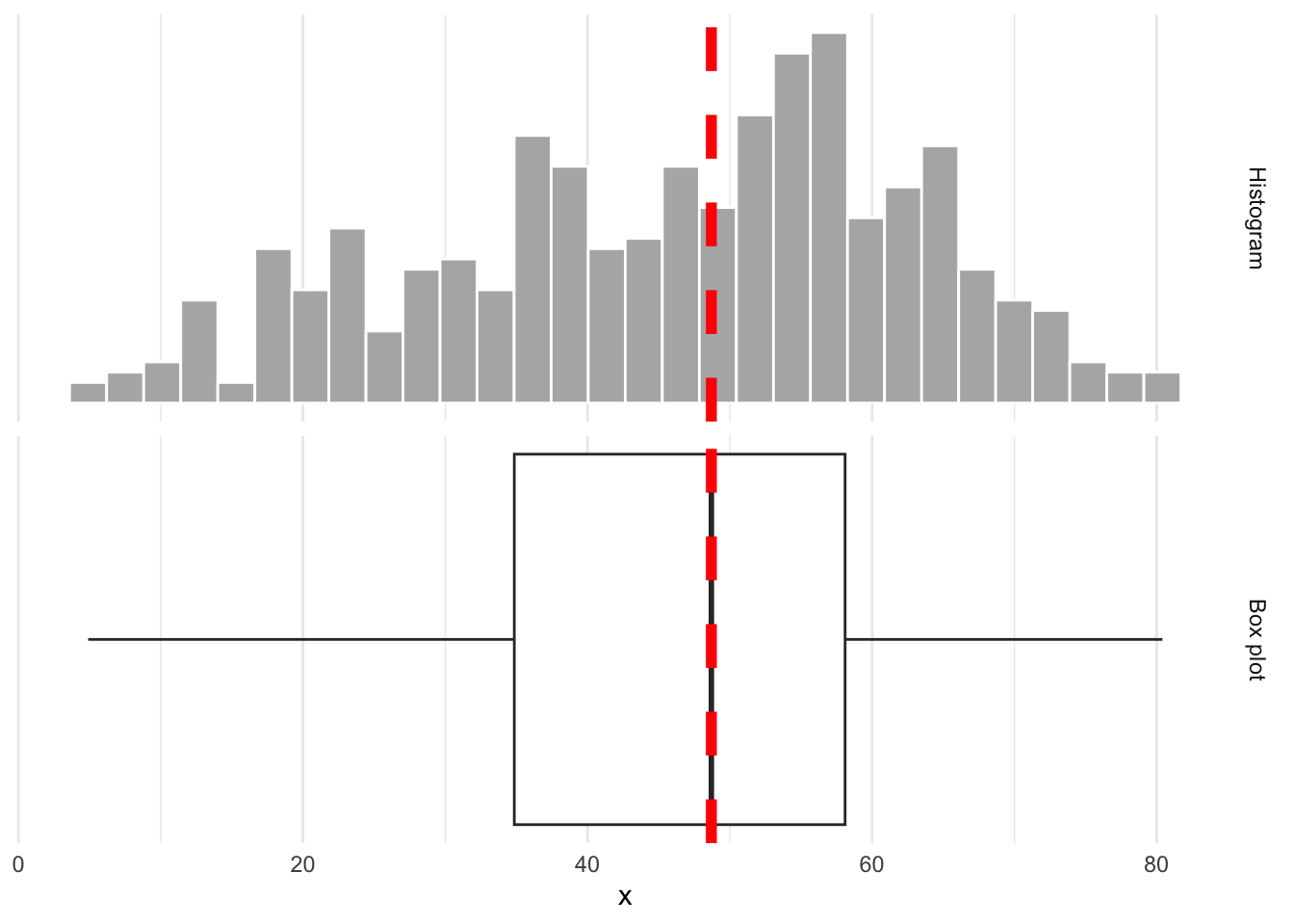
The middle of the box is the median. 50% of the data are below, and 50% are above:
Whence the box?
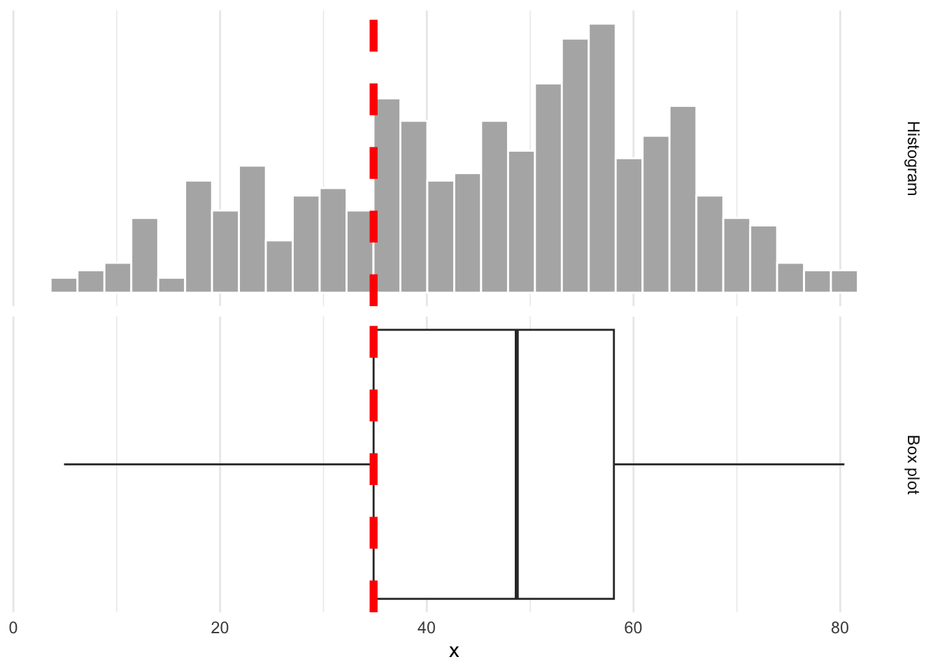
The lower edge of the box is the 25% quantile. 25% of the data are below, and 75% are above:
Whence the box?
The upper edge of the box is the 75% quantile. 75% of the data are below, and 25% are above:
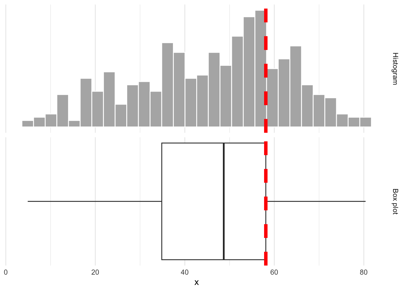
Box plot facts
- A box plot is easier to read quickly than a histogram because it eliminates clutter and immediately draws your eye to those main features: center, spread, and skew;
- The box spans the middle 50% of the data;
- The width of the box is called the inner quartile range (IQR) and it measures spread;
- From the docs (
?geom_boxplot):
The upper whisker extends from the hinge to the largest value no further than 1.5 * IQR from the hinge (where IQR is the inter-quartile range, or distance between the first and third quartiles). The lower whisker extends from the hinge to the smallest value at most 1.5 * IQR of the hinge. Data beyond the end of the whiskers are called “outlying” points and are plotted individually.
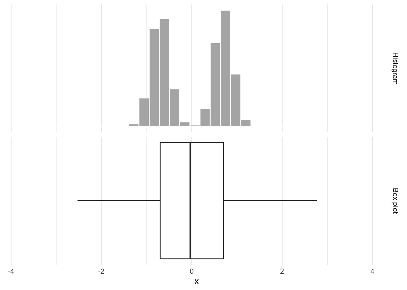
Box plots obscure modality
Same box plot:
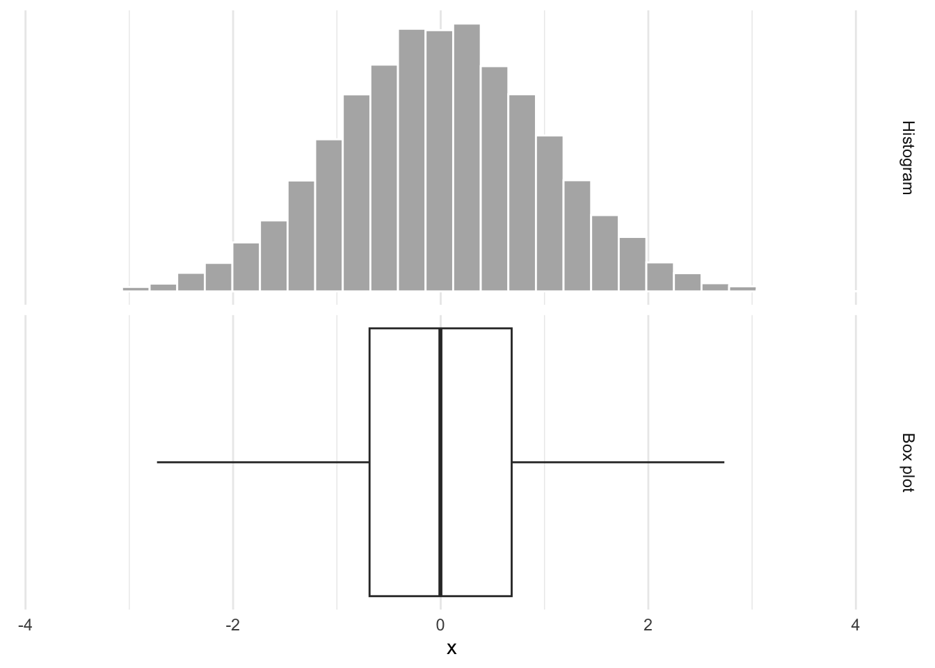
Box plots obscure modality
Very different distributions:
Density plot - Step 1
ggplot(gerrymander)
Density plot - Step 2

Density plot - Step 3
Contrast that with the histogram
ggplot(gerrymander, aes(x = trump16)) +
  geom_histogram(aes(y = after_stat(density))) +
  geom_density(color = "red")
`stat_bin()` using `bins = 30`. Pick better value `binwidth`.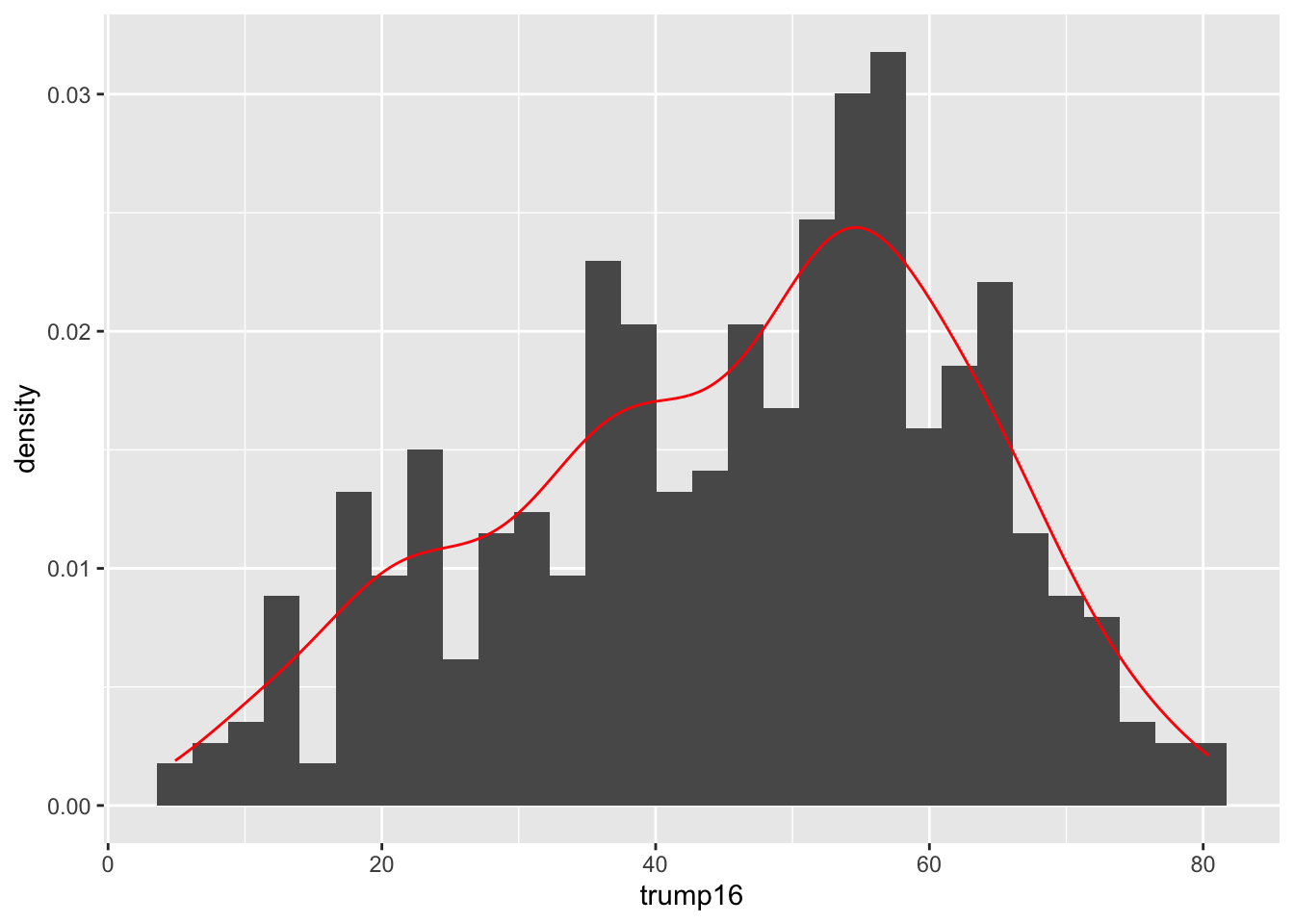
Prettier. Smooths out the lumps and bumps. There are still defaults you could learn to override.
Density plot - Step 4
ggplot(gerrymander, aes(x = trump16)) +
  geom_density(color = "red")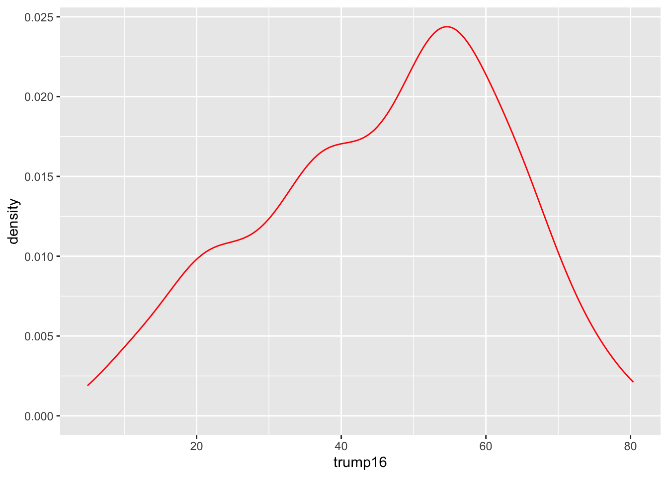
Density plot - Step 5
ggplot(gerrymander, aes(x = trump16)) +
  geom_density(color = "firebrick", fill = "firebrick1")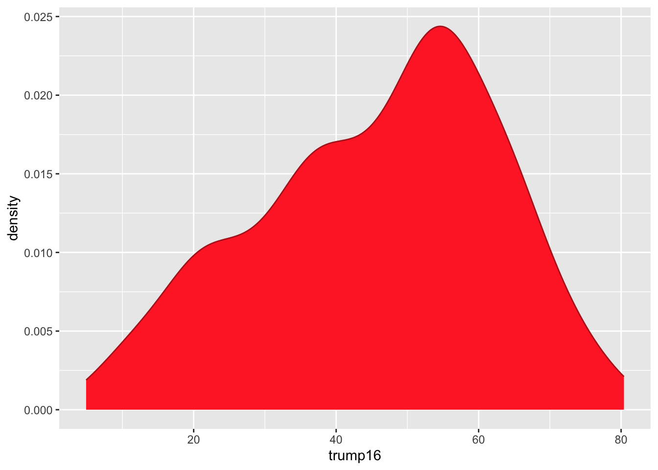
Density plot - Step 6
ggplot(gerrymander, aes(x = trump16)) +
  geom_density(color = "firebrick", fill = "firebrick1", alpha = 1)
Density plot - Step 6
ggplot(gerrymander, aes(x = trump16)) +
  geom_density(color = "firebrick", fill = "firebrick1", alpha = 0)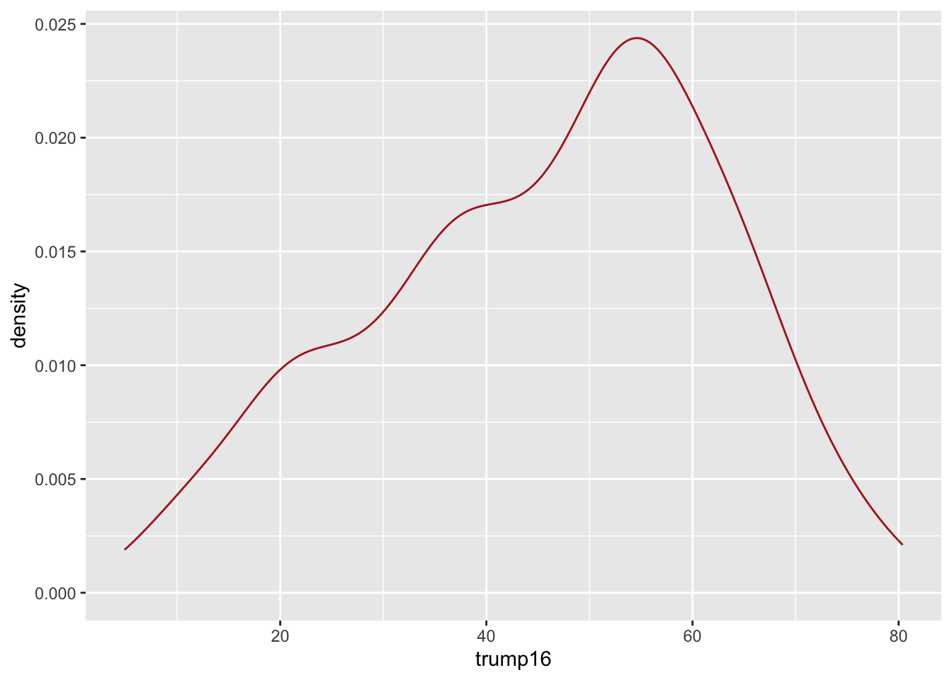
Density plot - Step 6
ggplot(gerrymander, aes(x = trump16)) +
  geom_density(color = "firebrick", fill = "firebrick1", alpha = 0.5)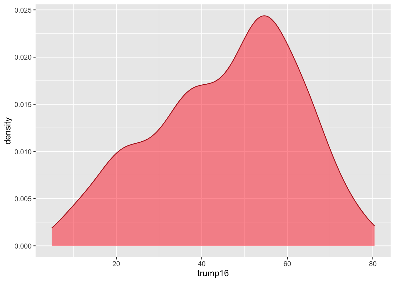
Density plot - Step 7
ggplot(gerrymander, aes(x = trump16)) +
  geom_density(color = "firebrick", fill = "firebrick1", alpha = 0.5, linewidth = 2)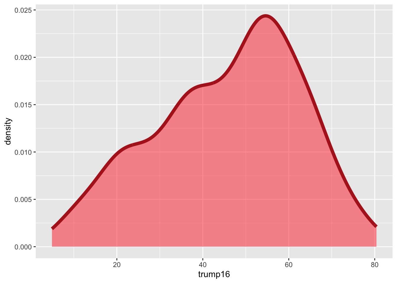
Density plot - Step 8
Summary statistics
gerrymander |>
  summarize(
    mean_trump_perc = mean(trump16),
    median_trump_perc = median(trump16),
    sd = sd(trump16),
    iqr = IQR(trump16),
    q25 = quantile(trump16, 0.25),
    q75 = quantile(trump16, 0.75)
  )
# A tibble: 1 × 6
mean_trump_perc median_trump_perc sd iqr q25 q75
<dbl> <dbl> <dbl> <dbl> <dbl> <dbl>
1 45.9 48.7 16.8 23.3 34.8 58.1What does this code do?
# A tibble: 1 × 2
  gimme_my_mean gimme_my_median
          <dbl>           <dbl>
1 45.9 48.7-
summarizecreates a new data frame that stores the summaries; - You can compute as many summaries as you want;
- To the left of the equal signs are your choice of column names in the new data frame you are creating. You can type whatever you want here (within reason);
- To the right of the equal signs is
Rcode that computes the summaries. You must use the correct command names (case sensitive):mean,median,quantile,sd,var, etc; - If you want to learn what these do, read the documentation (eg
?quantile).
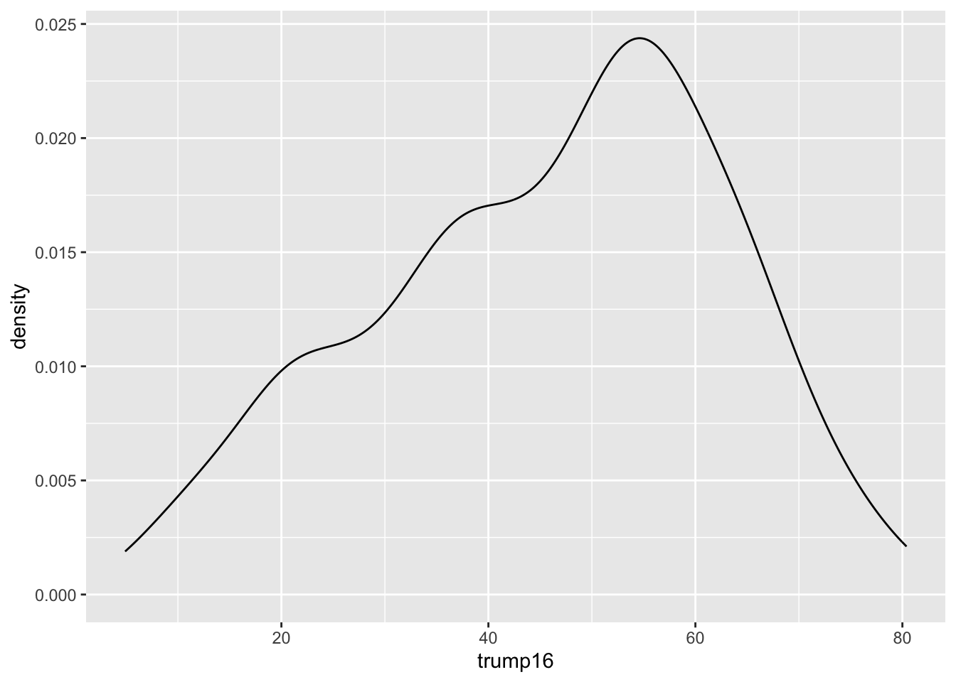
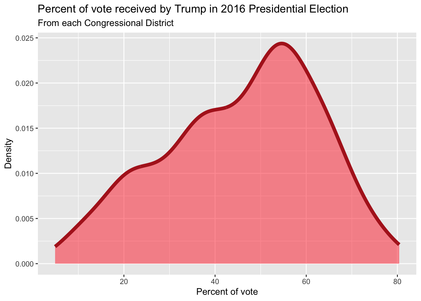
Distribution of votes for Trump in the 2016 election
Describe the distribution of percent of vote received by Trump in 2016 Presidential Election from Congressional Districts.
Shape: The distribution of votes for Trump in the 2016 election from Congressional Districts is unimodal and left-skewed.
Center: The percent of vote received by Trump in the 2016 Presidential Election from a typical Congressional Districts is 48.7%.
Spread: In the middle 50% of Congressional Districts, 34.8% to 58.1% of voters voted for Trump in the 2016 Presidential Election.
Unusual observations: -
Bivariate analysis
Bivariate analysis
Analyzing the relationship between two variables:
Numerical + numerical: scatterplot
Numerical + categorical: side-by-side box plots, violin plots, etc.
Categorical + categorical: stacked bar plots
Using an aesthetic (e.g., fill, color, shape, etc.) or facets to represent the second variable in any plot
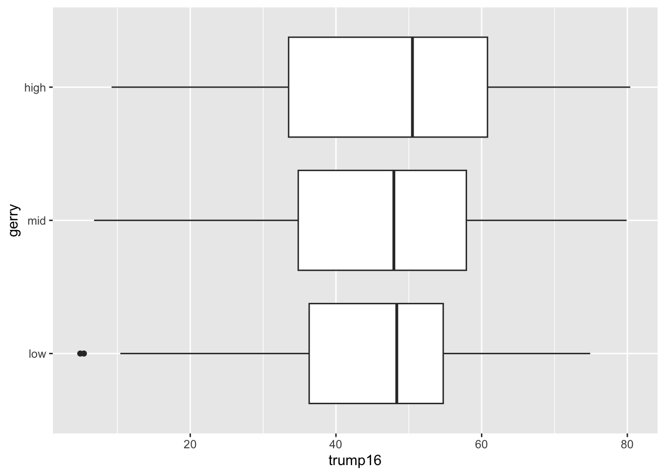
Side-by-side box plots
Summary statistics
Summary statistics
Summary statistics
Summary statistics
Summary statistics
gerrymander |>
  group_by(gerry) |>
  summarize(
    min = min(trump16),
    q25 = quantile(trump16, 0.25),
    median = median(trump16),
    q75 = quantile(trump16, 0.75),
    max = max(trump16),
  )
# A tibble: 3 × 6
gerry min q25 median q75 max
<fct> <dbl> <dbl> <dbl> <dbl> <dbl>
1 low 4.9 36.3 48.4 54.7 74.9
2 mid 6.8 34.8 48.0 57.9 79.9
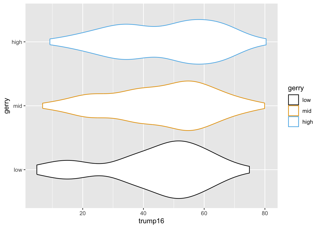
3 high 9.2 33.5 50.5 60.8 80.4Density plots
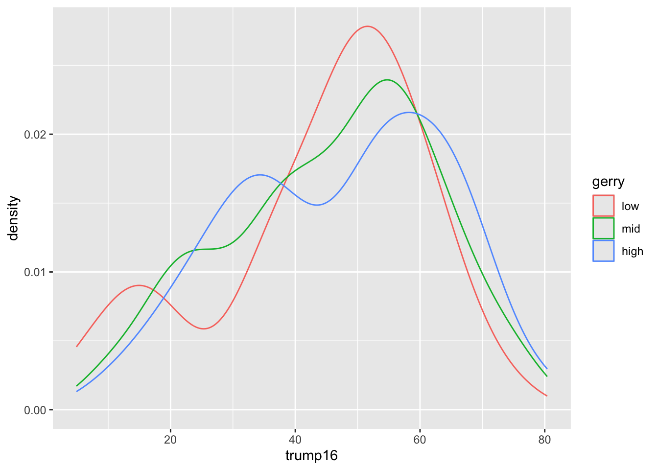
Filled density plots
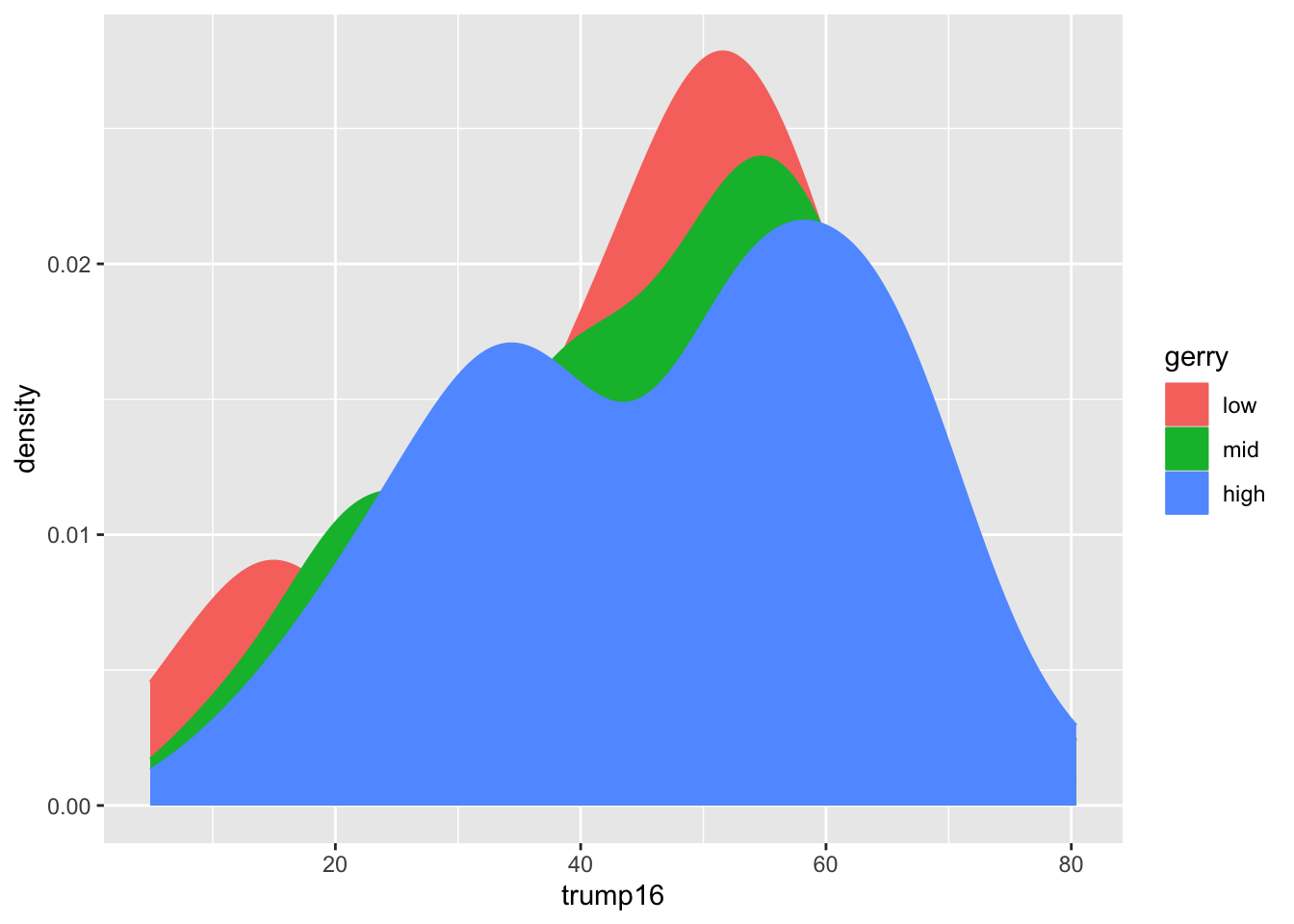
Better filled density plots
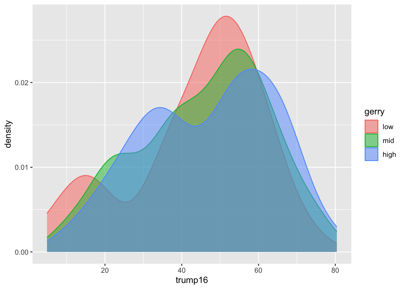
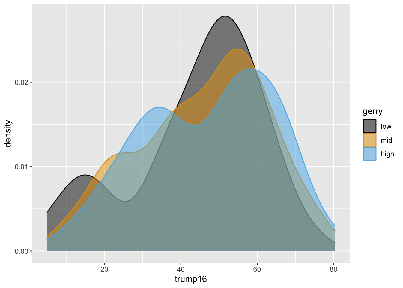
Better colors
Violin plots
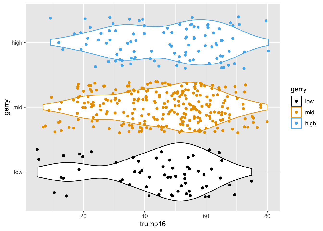
Multiple geoms
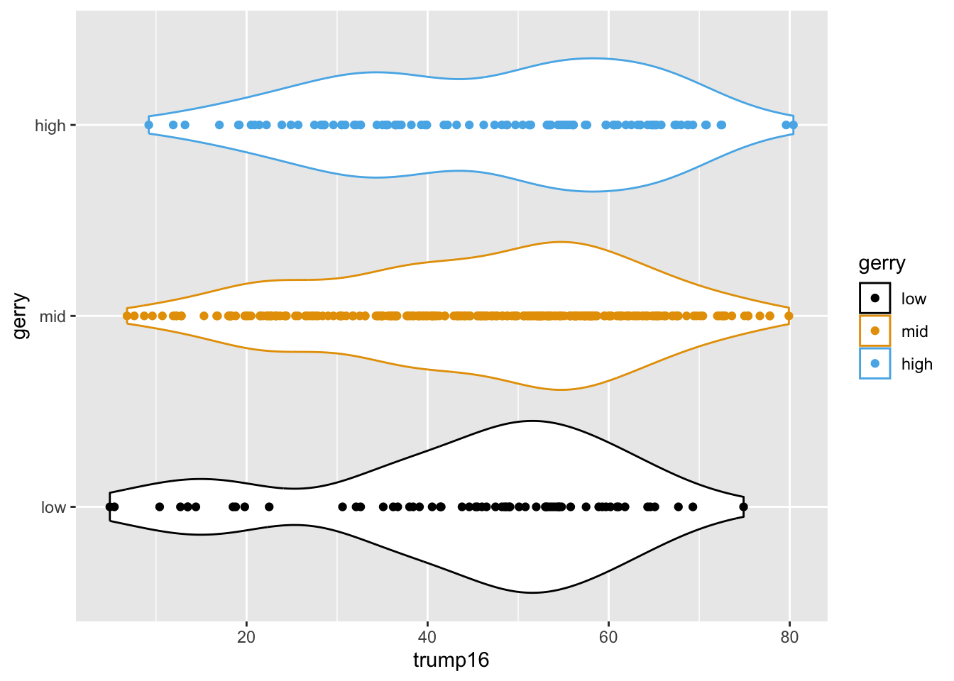
Multiple geoms
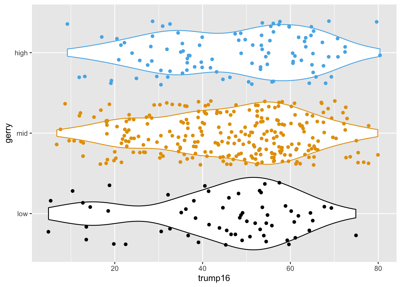
Remove legend
Multivariate analysis
Multivariate analysis
Analyzing the relationship between multiple variables:
In general, one variable is identified as the outcome of interest
The remaining variables are predictors or explanatory variables
-
Plots for exploring multivariate relationships are the same as those for bivariate relationships, but conditional on one or more variables
- Conditioning can be done via faceting or aesthetic mappings (e.g., scatterplot of
yvs.x1, colored byx2, faceted byx3)
- Conditioning can be done via faceting or aesthetic mappings (e.g., scatterplot of
-
Summary statistics for exploring multivariate relationships are the same as those for bivariate relationships, but conditional on one or more variables
- Conditioning can be done via grouping (e.g., correlation between
yandx1, grouped by levels ofx2andx3)
- Conditioning can be done via grouping (e.g., correlation between
Application exercise
ae-04-gerrymander-explore-I
Go to your ae project in RStudio.
If you haven’t yet done so, make sure all of your changes up to this point are committed and pushed, i.e., there’s nothing left in your Git pane.
If you haven’t yet done so, click Pull to get today’s application exercise file: ae-04-gerrymander-explore-I.qmd.
Work through the application exercise in class, and render, commit, and push your edits by the end of class.