Interval estimation
Lecture 22
While you wait: Participate 📱💻
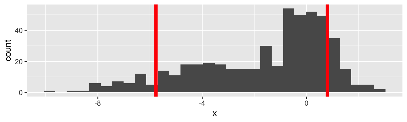
The line on the left is the 8% quantile of the data, and the line on the right is the 87% quantile of the data. What fraction of the data lives between the two lines?
- 50%
- 79%
- 80%
- 87%
- 95%
Scan the QR code or go HERE. Log in with your Duke NetID.
Admin
The home stretch
- Monday April 13: lecture on confidence intervals;
- Wednesday April 15: lecture on hypothesis testing;
- Thursday April 16: graded lab on statistics (last one!);
- Monday April 20: wrap-up lecture on inference;
- Wednesday April 22: lecture on who knows what (last one!);
- Wednesday April 22: turn in HW 7 (last one!);
- Friday May 1 : final exam @ 2pm.
On the horizon
- Project grades posted this week
- Midterm 2 grades posted this week
- After Wednesday April 22: drop four days from attendance score
- After Lab 8 is graded: drop two lowest labs
- After HW 7 is graded: drop lowest HW
- 80% of your final course grade is locked going into the final
- I replace your lowest midterm score (the whole thing) with your final exam score, if it’s better
Also

Statistics
The bottom line, at the top
If JZ had to boil statistics down to one main idea, it would be:
quantifying uncertainty to help make decisions.
You make different kinds of decisions if you’re sure versus unsure. Statistics helps you quantify the reliability of your knowledge so that you can determine what sort of decision to make.
Quantifying uncertainty to help make decisions
- What kind of uncertainty?
- How do you quantify it?
- These are surprisingly spicy and controversial questions in statistics!
- With the short time remaining, we will focus on quantifying one specific type of uncertainty…
Classical sampling uncertainty
Sampling uncertainty
Different data give different estimates. How different?
- In reality, we have one dataset, and it gives one set of results. How reliable are those results?
- A thought experiment: if I collected a whole new dataset and redid my analysis, do I get the same results, or different results?
- if the results vary wildly from dataset to dataset, uncertainty is high and reliability is low;
- if the results are stable from one dataset to another, uncertainty is low and reliability is high.
That’s the main idea in a nutshell.
A running example
Recall the openintro::loans_full_schema data frame:
10000 rows;
each row is an approved loan applicant;
-
the columns contain financial info about that person, including…
- annual income (in $);
- amount of non-mortgage debt outstanding (in $).
What would you guess is the direction of association between these two variables?
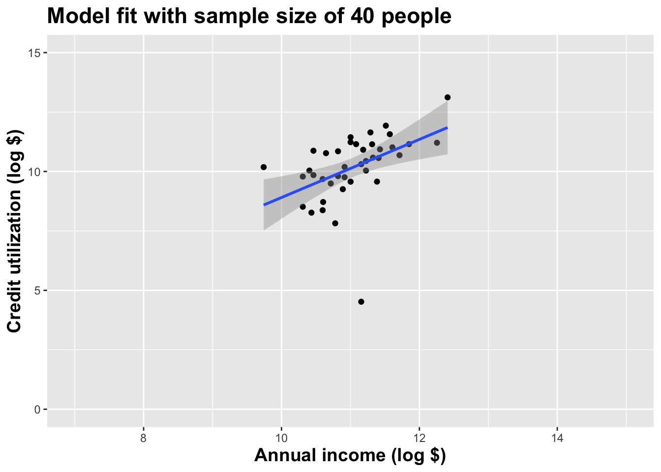
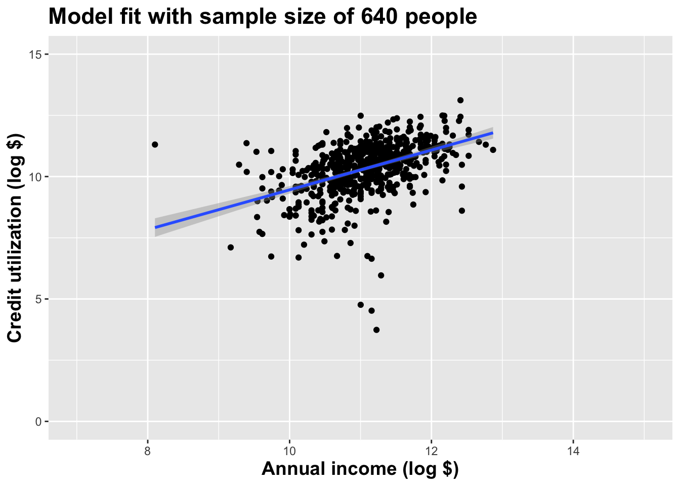
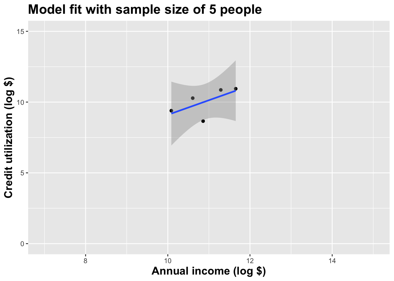
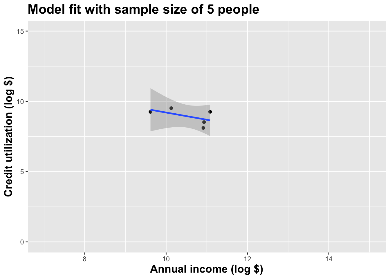
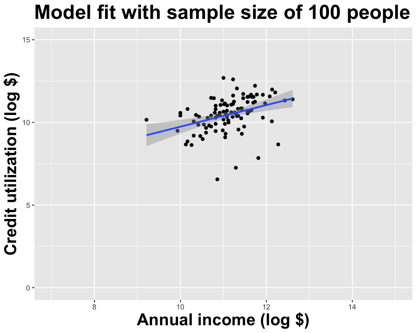
Model fit with five observations
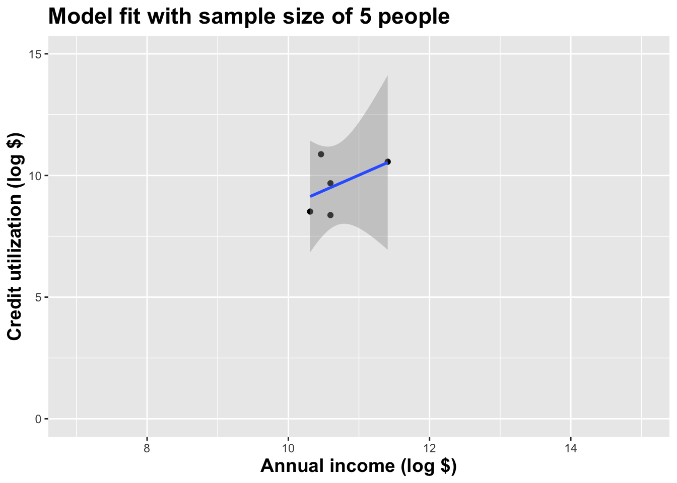
(I just took logs to make the picture prettier.)
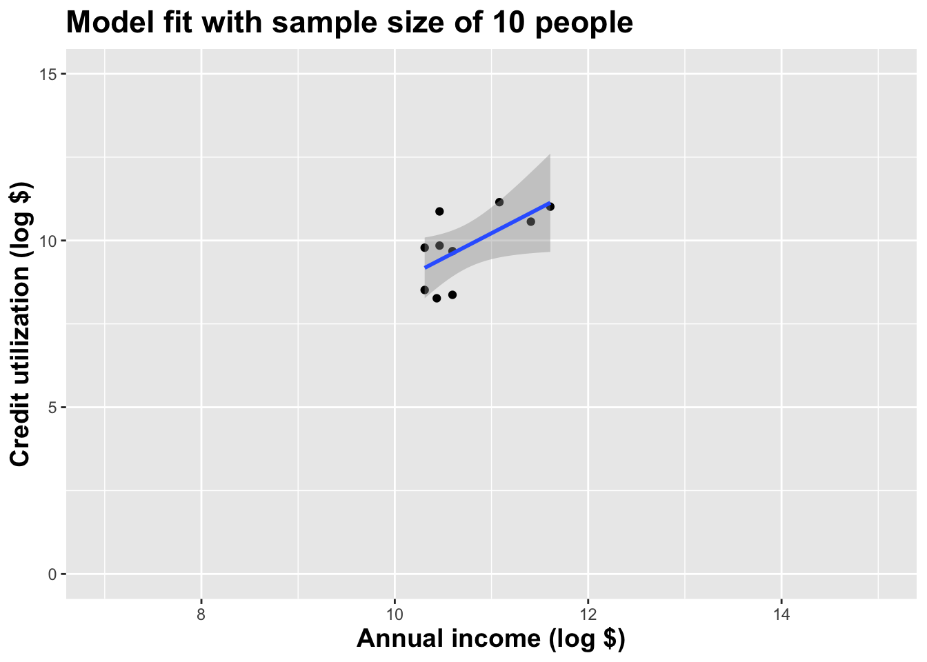
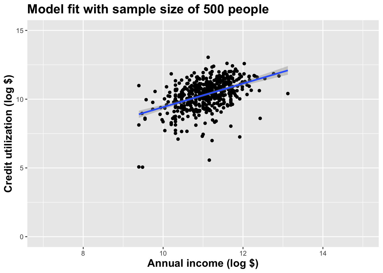
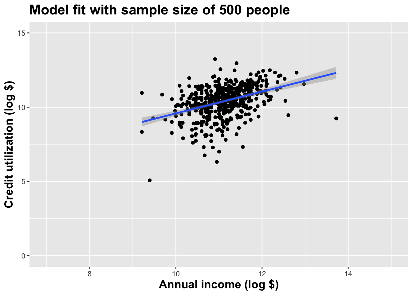
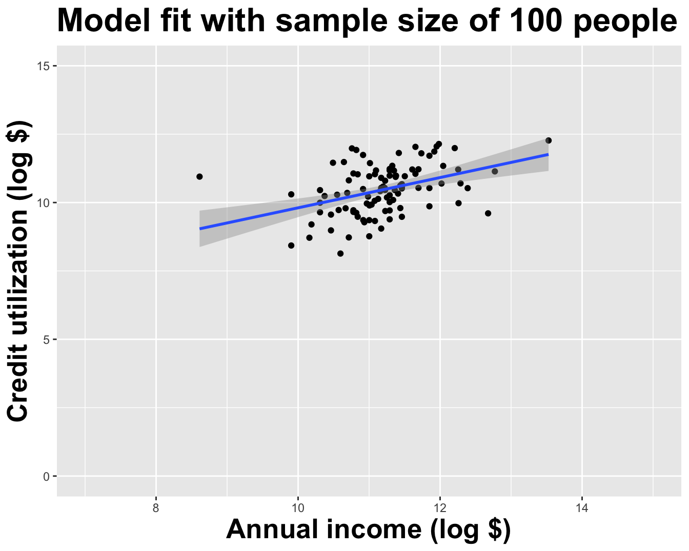
Double the sample size
Double the sample size again
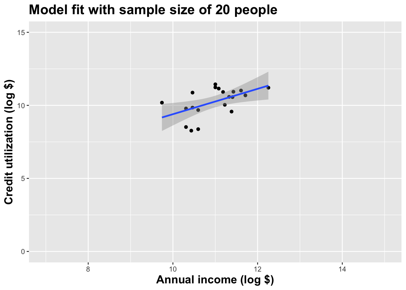
Double the sample size again
Double the sample size again
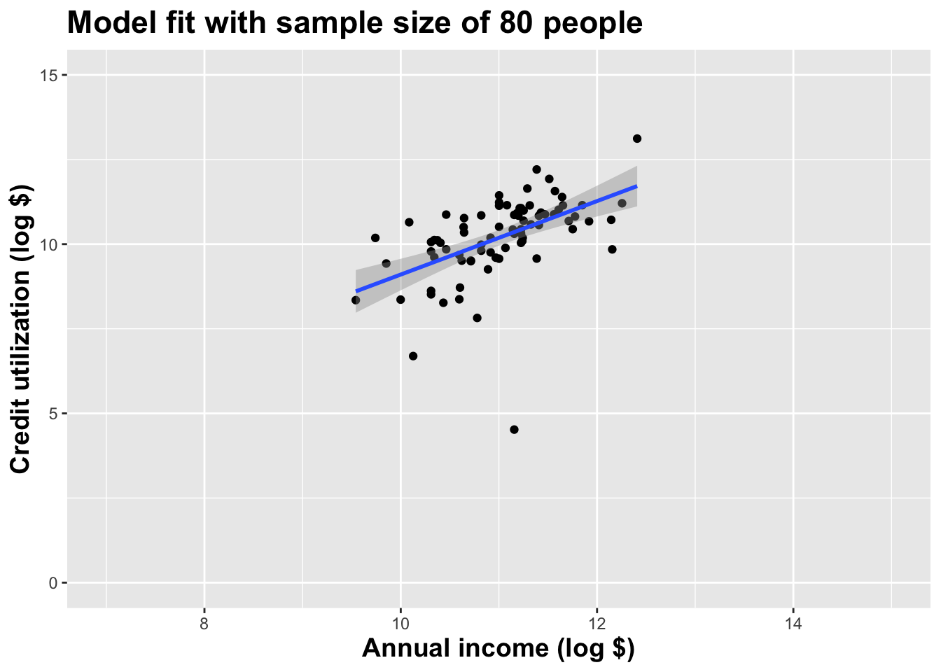
Double the sample size again
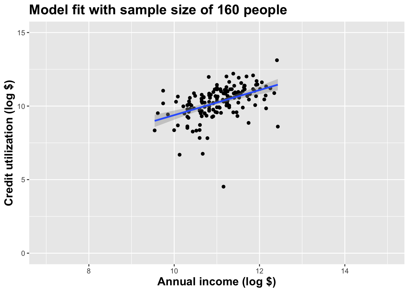
Double the sample size again
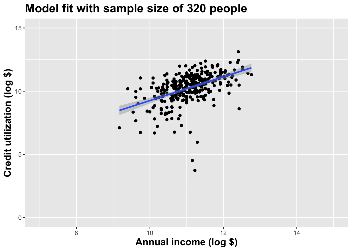
Double the sample size again
Double the sample size again
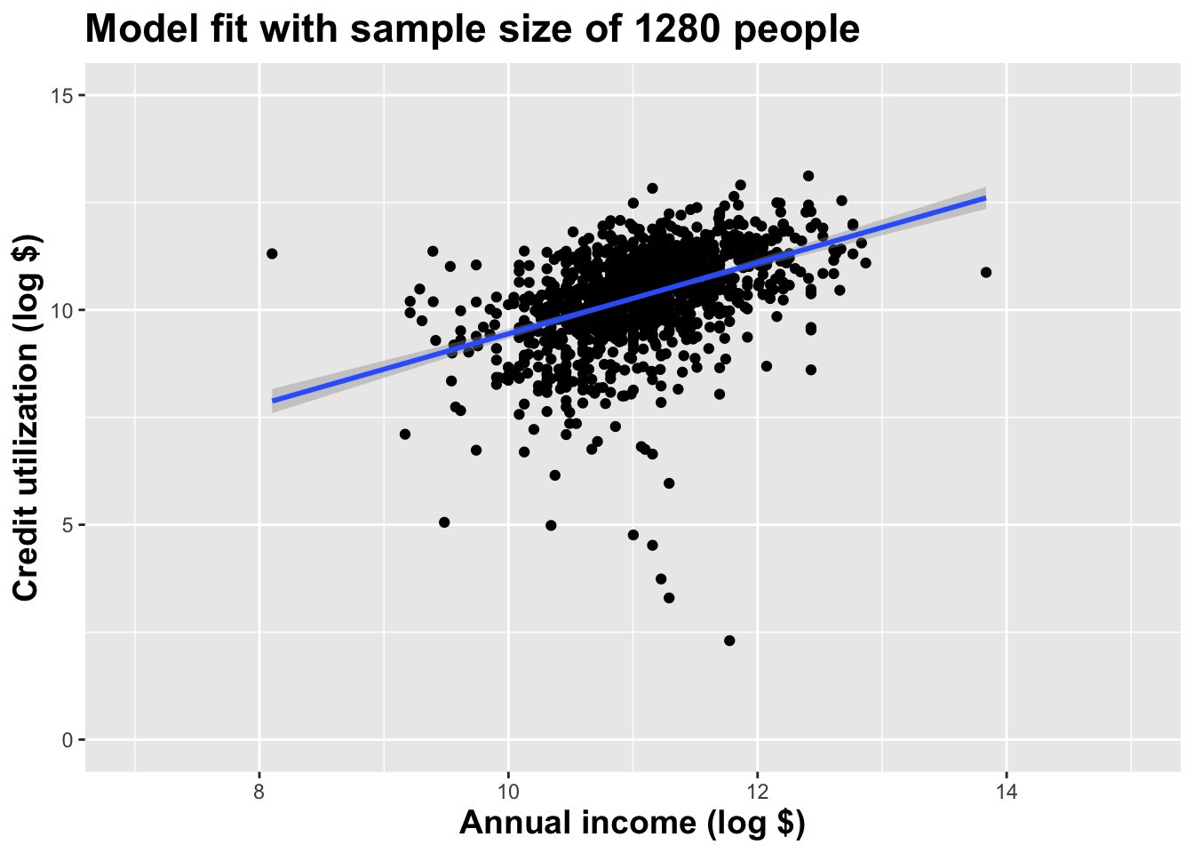
Double the sample size yet again
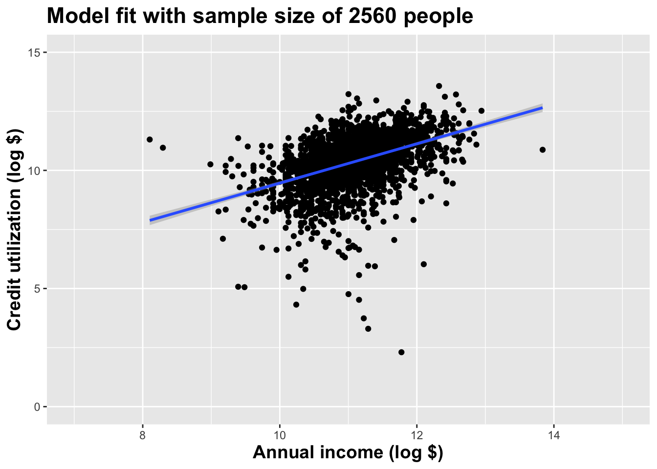
Double the sample size one more time
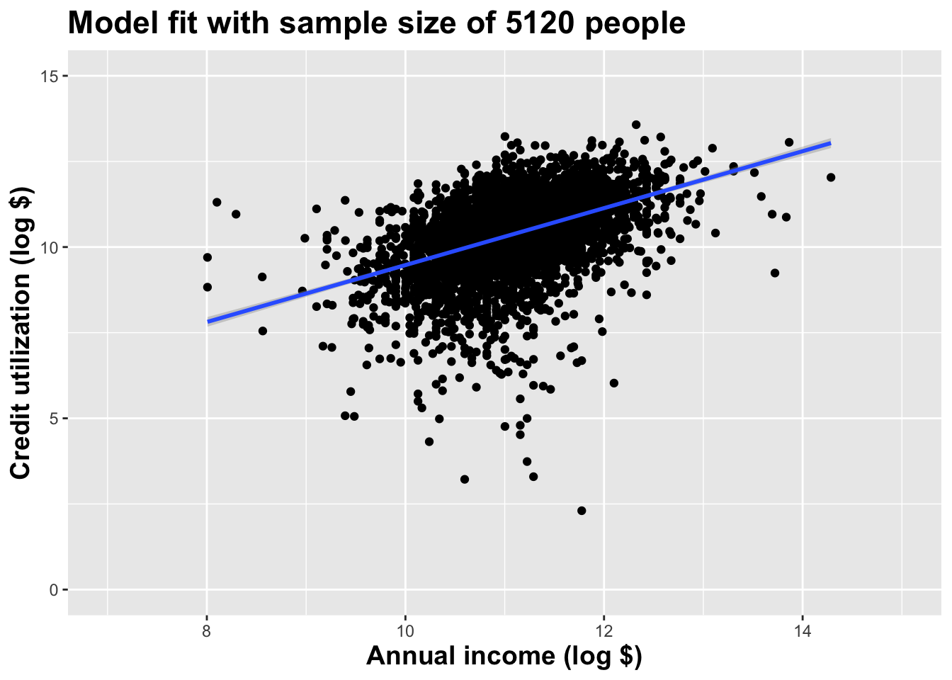
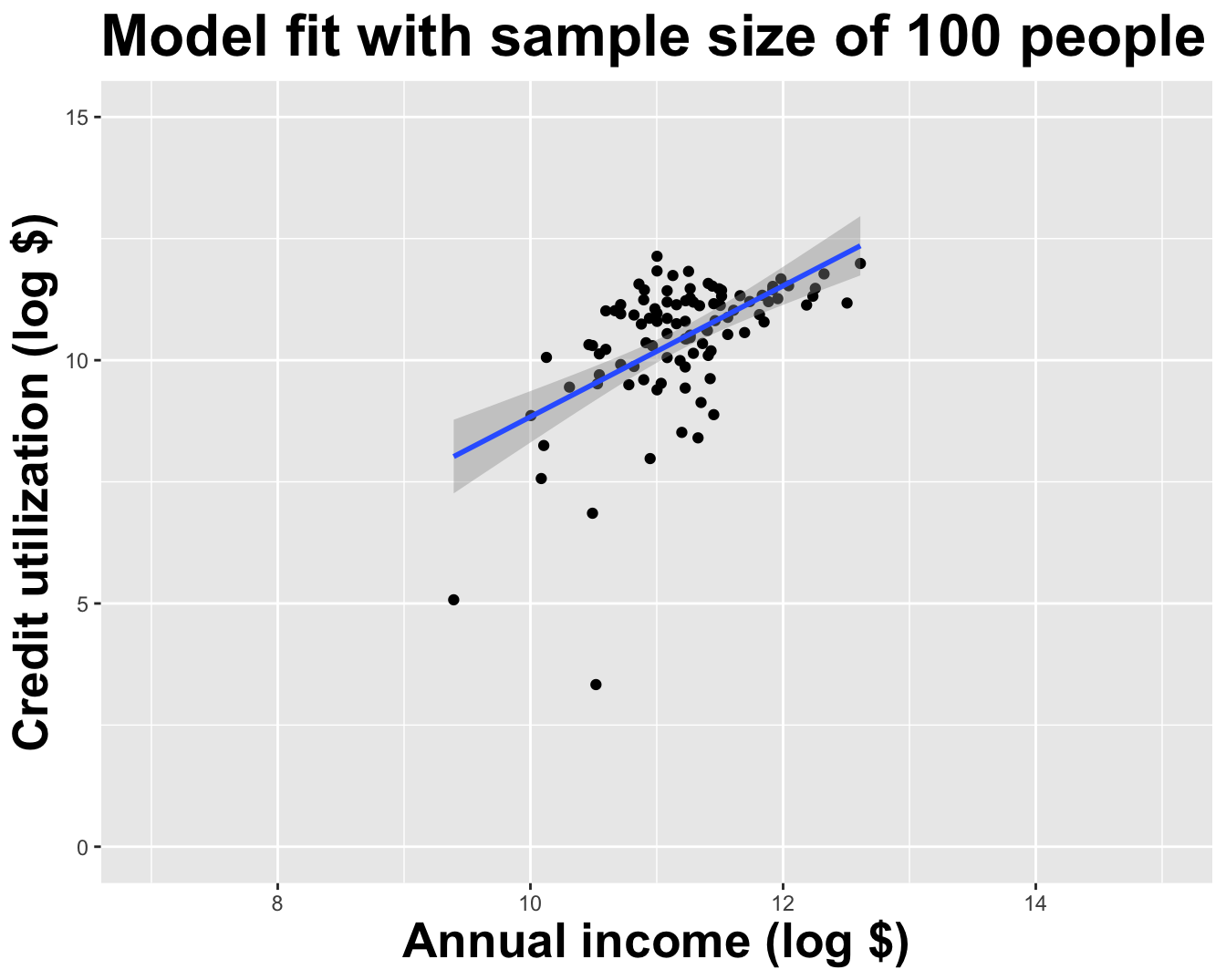
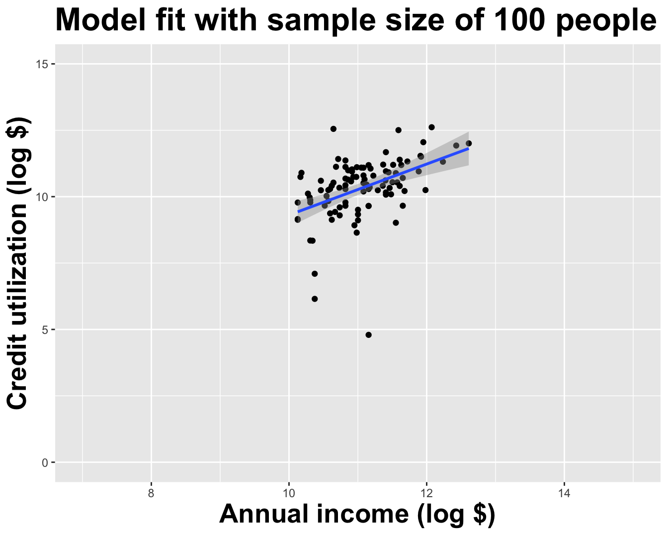
Use all the data we have
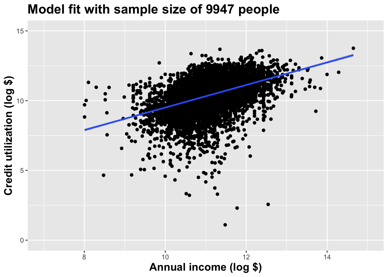
What did we notice?
As the sample size grew, the best fit line stabilized;
As the sample size grew, the grey uncertainty band shrank;
As the sample size grew, we observed a larger range of income values, anf the computer displayed more of the line;
-
As the sample size grows, the picture the data paint becomes clearer:
- positive relationship;
- linear relationship;
- pretty strong
A silly question
Which would you rather have for your data analysis? 5 people in your dataset or 9947? Why?
Here’s the deal
We do not know what the “true” line is;
Our estimates are a best guess based on noisy, incomplete, imperfect data;
The more data we have, the more “certain” and “reliable” the estimates are;
What do we mean by “uncertainty” here?
Sampling uncertainty
Fact: different data set -> different estimates;
-
How much would our estimate vary across alternative datasets?
- If the answer is “a lot,” uncertainty is high, and our estimates are not super reliable;
- If the answer is “a little,” uncertainty is low, and maybe we can take our estimates to the bank;
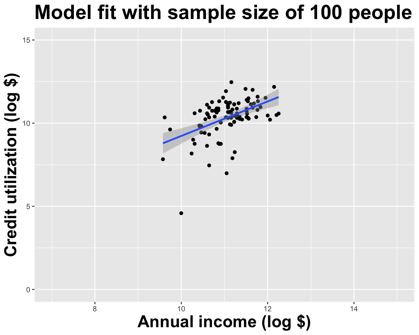
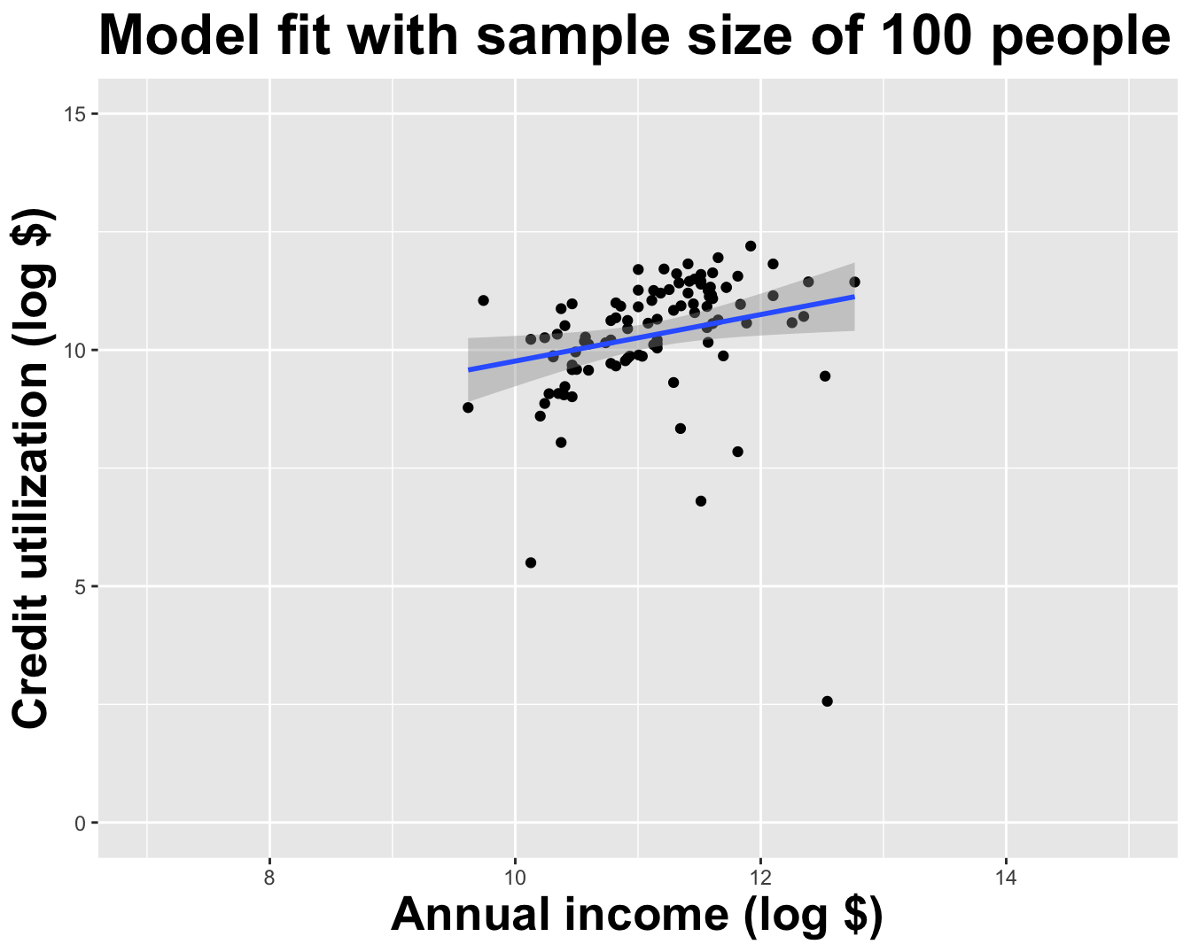
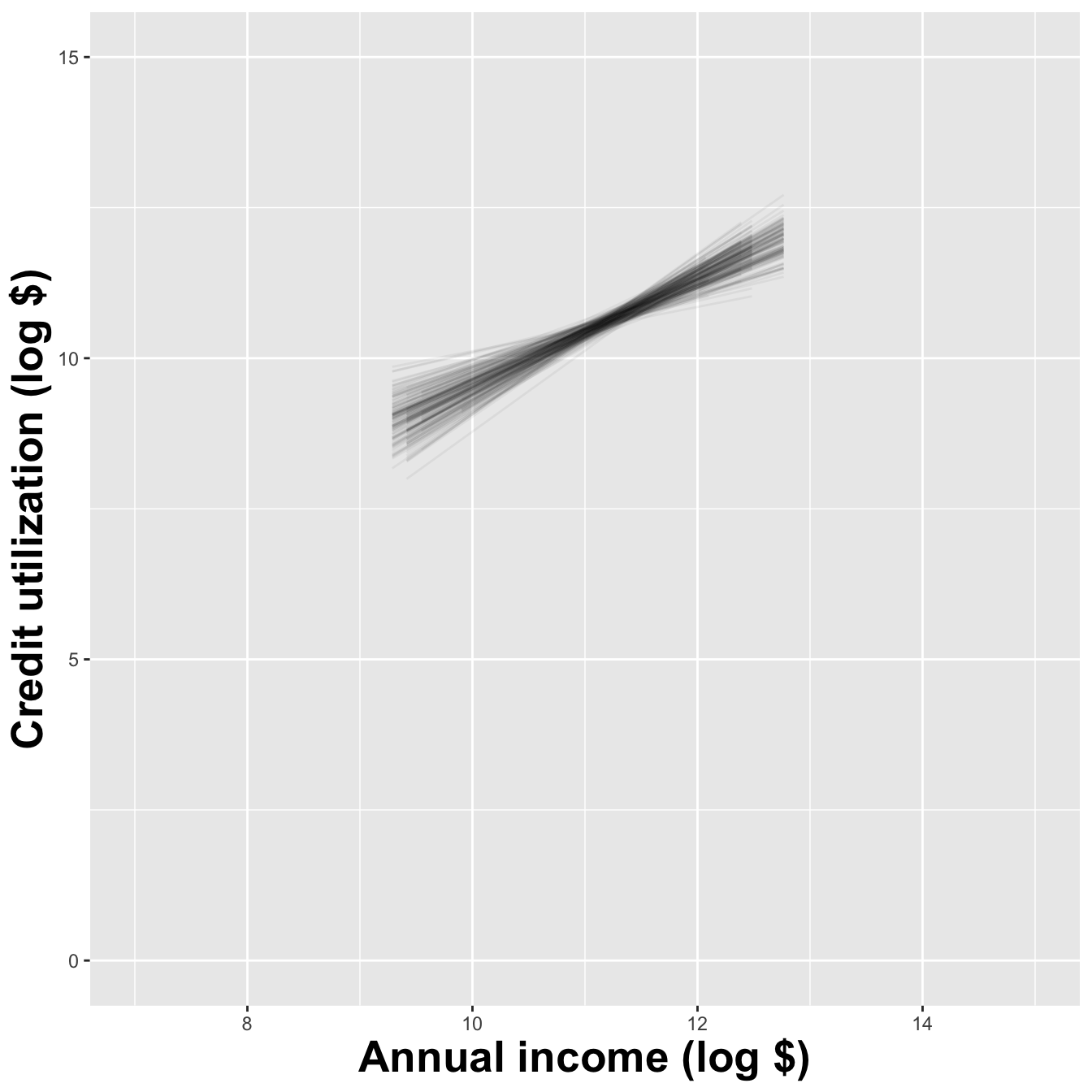
Here’s one dataset we could have seen
Here’s another
Here’s yet one more
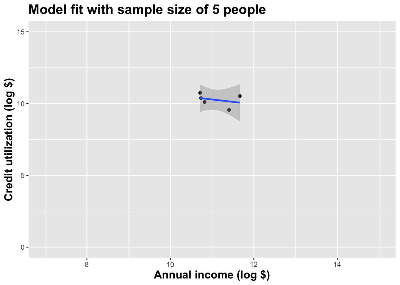
Different data set -> different estimates
These tiny data sets can’t even agree on if the line should slope up or down. Uncertainty is high, hence the large bands.
If we repeat the process with a larger sample size, things are more stable
Alternative 1
Alternative 2

Alternative 3
Let’s visualize how the estimates vary
Different data set -> different estimates
# A tibble: 2 × 2
  term        estimate
  <chr>          <dbl>
1 (Intercept)    4.27
2 log_inc        0.553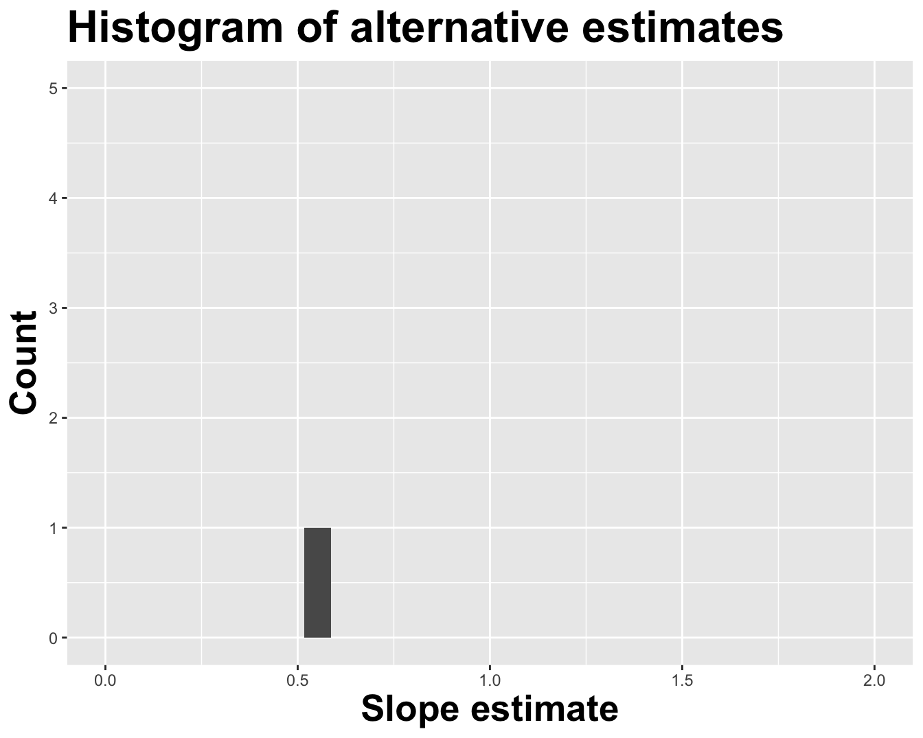
Different data set -> different estimates
# A tibble: 2 × 2
  term        estimate
  <chr>          <dbl>
1 (Intercept)    -4.63
2 log_inc         1.35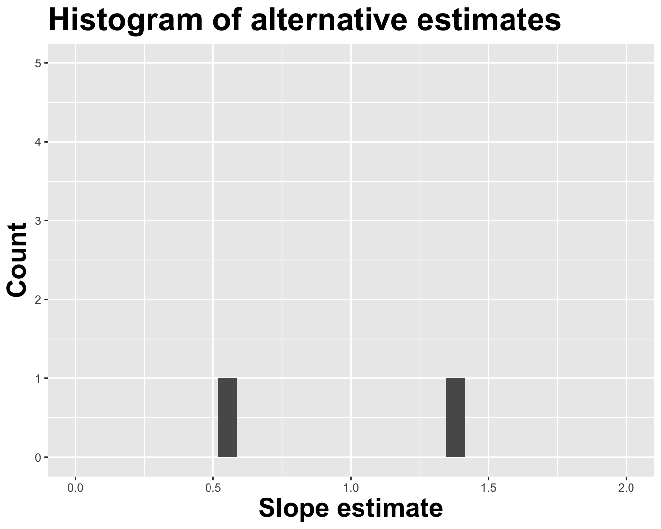
Different data set -> different estimates
# A tibble: 2 × 2
  term        estimate
  <chr>          <dbl>
1 (Intercept)    -1.14
2 log_inc         1.04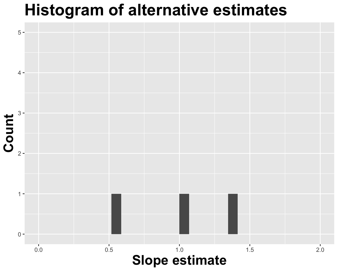
Different data set -> different estimates
# A tibble: 2 × 2
  term        estimate
  <chr>          <dbl>
1 (Intercept)   -0.288
2 log_inc        0.960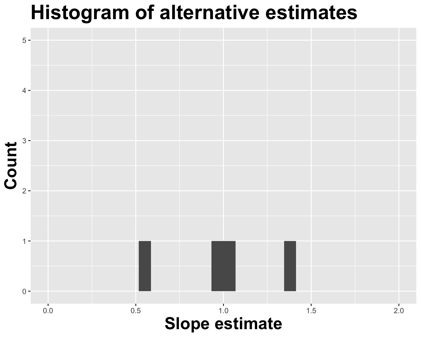
Different data set -> different estimates
# A tibble: 2 × 2
  term        estimate
  <chr>          <dbl>
1 (Intercept)    4.84
2 log_inc        0.492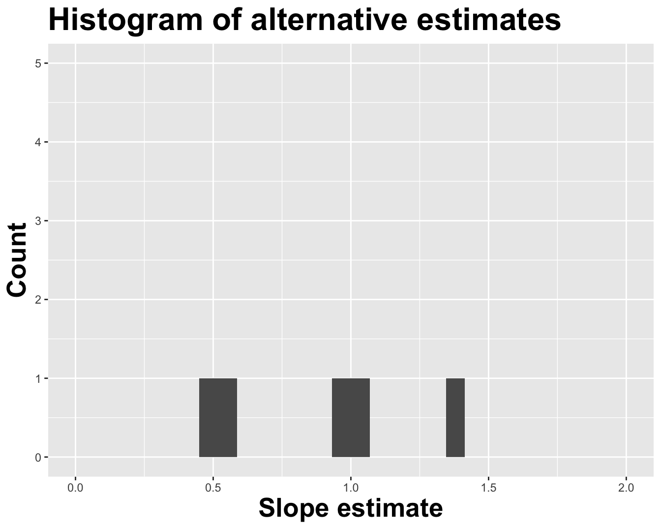
Different data set -> different estimates
# A tibble: 2 × 2
  term        estimate
  <chr>          <dbl>
1 (Intercept)    3.20
2 log_inc        0.654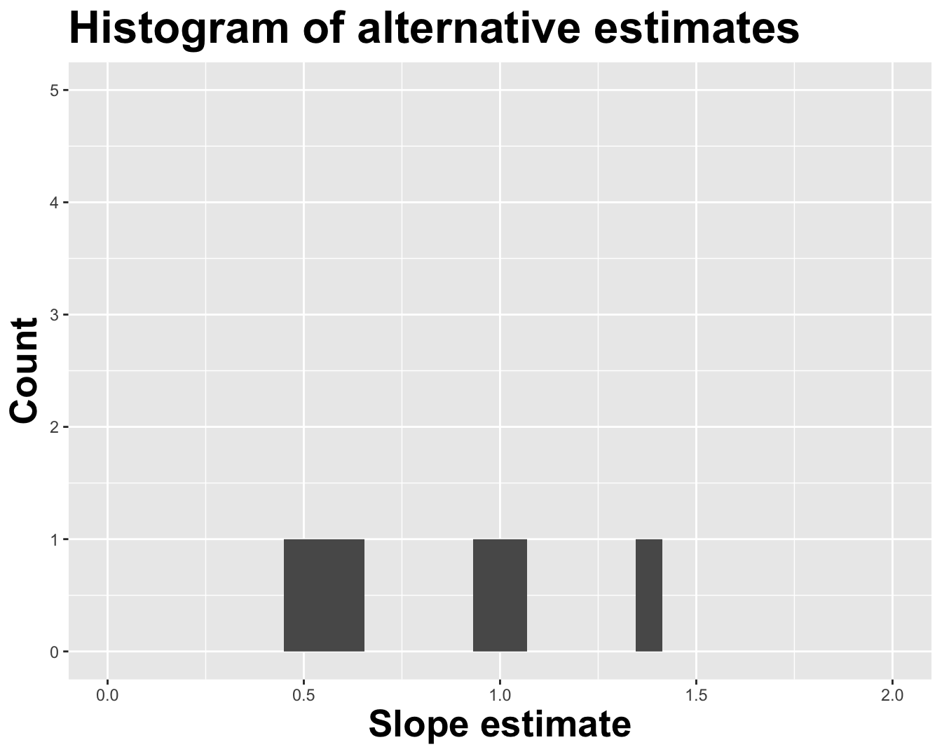
You get the idea

Variation in estimates across alternative datasets
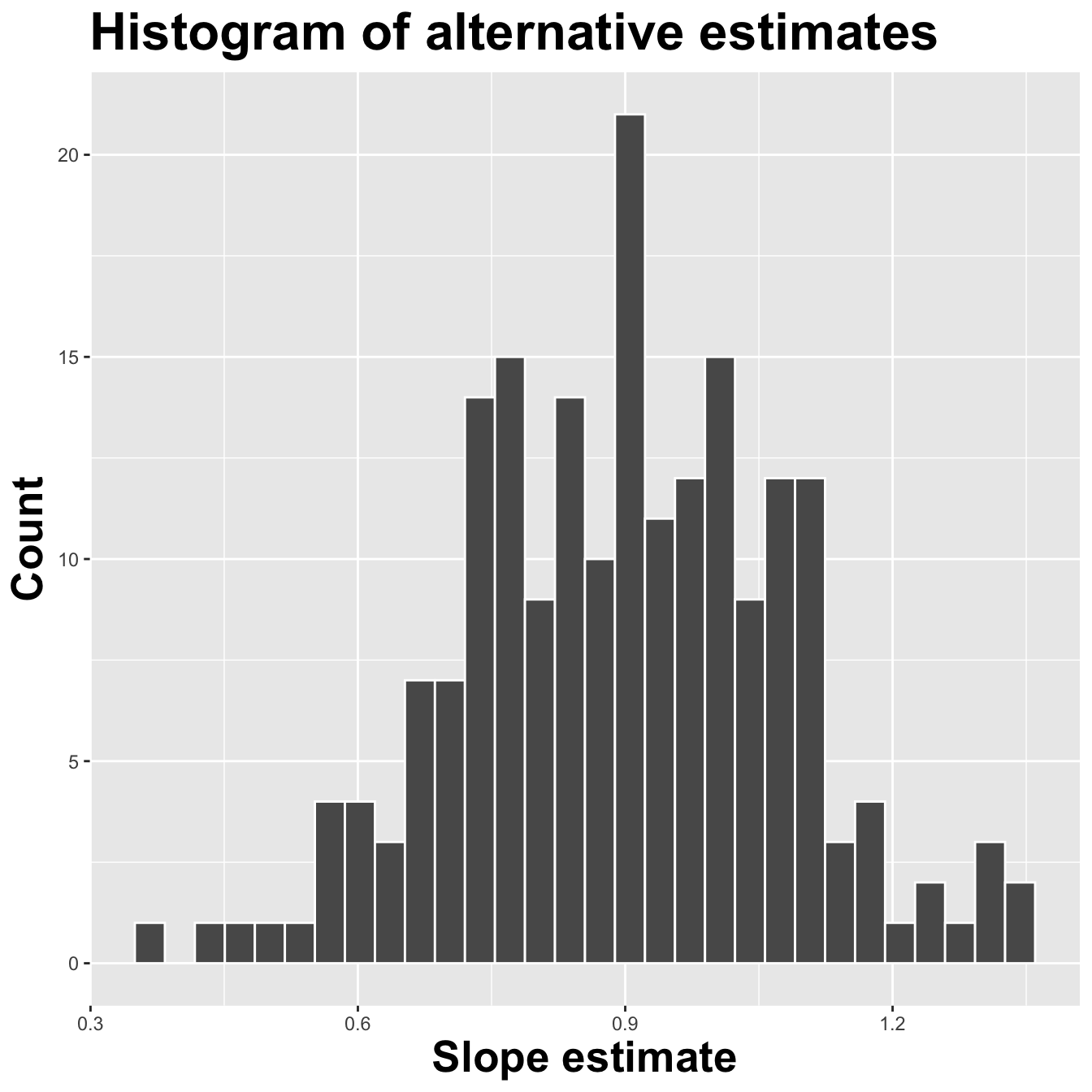
The amount of variation in the histogram tells us something about the uncertainty, and gives us a range of likely values.
Summary
- The notion of uncertainty we seek to quantify is “variability of estimates across datasets;”
- If the estimates vary a lot across datasets, reliability is low and uncertainty is high;
- If the estimates vary only a little across datasets, reliability is high and uncertainty is low;
- We can visualizes this with a histogram of estimates, and quantify it with the spread of that histogram (sd, var, IQR, etc);
- Sampling uncertainty is influenced by the underlying noisiness of the data and the sample size.
. . .
In order to do this in practice, we need multiple datasets. But in practice we only have one. So now what?
The bootstrap
Reality check
- Contemplating alternative datasets is a cute thought experiment, but in reality we cannot collect completely new data;
- Data collection is costly!
- Collecting new survey responses;
- Recruiting new subjects;
- Running new experiments;
- Firing up the Large Hadron Collider for one more go;
- Given the one dataset we actually have, how can we approximate the idea of alternative datasets and use them to assess the variability of results?
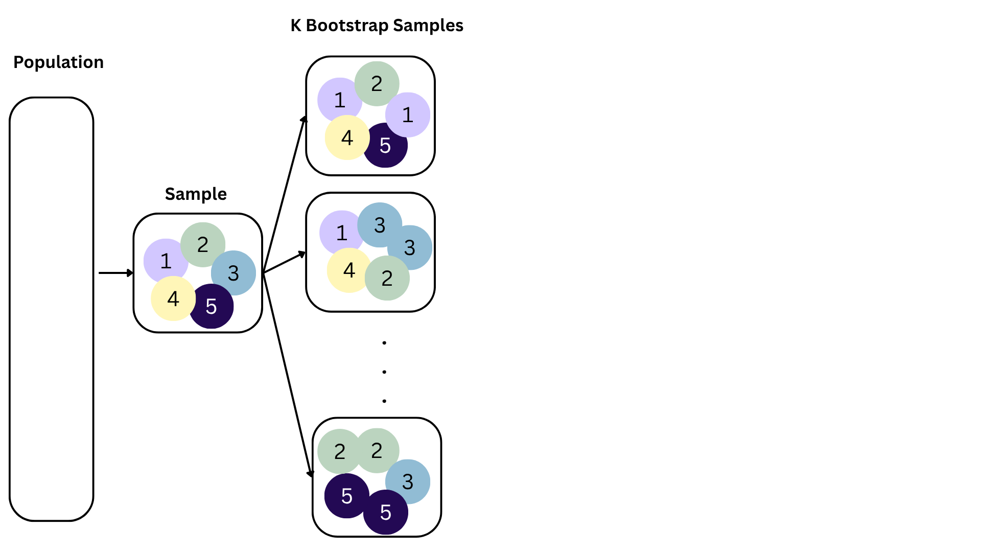
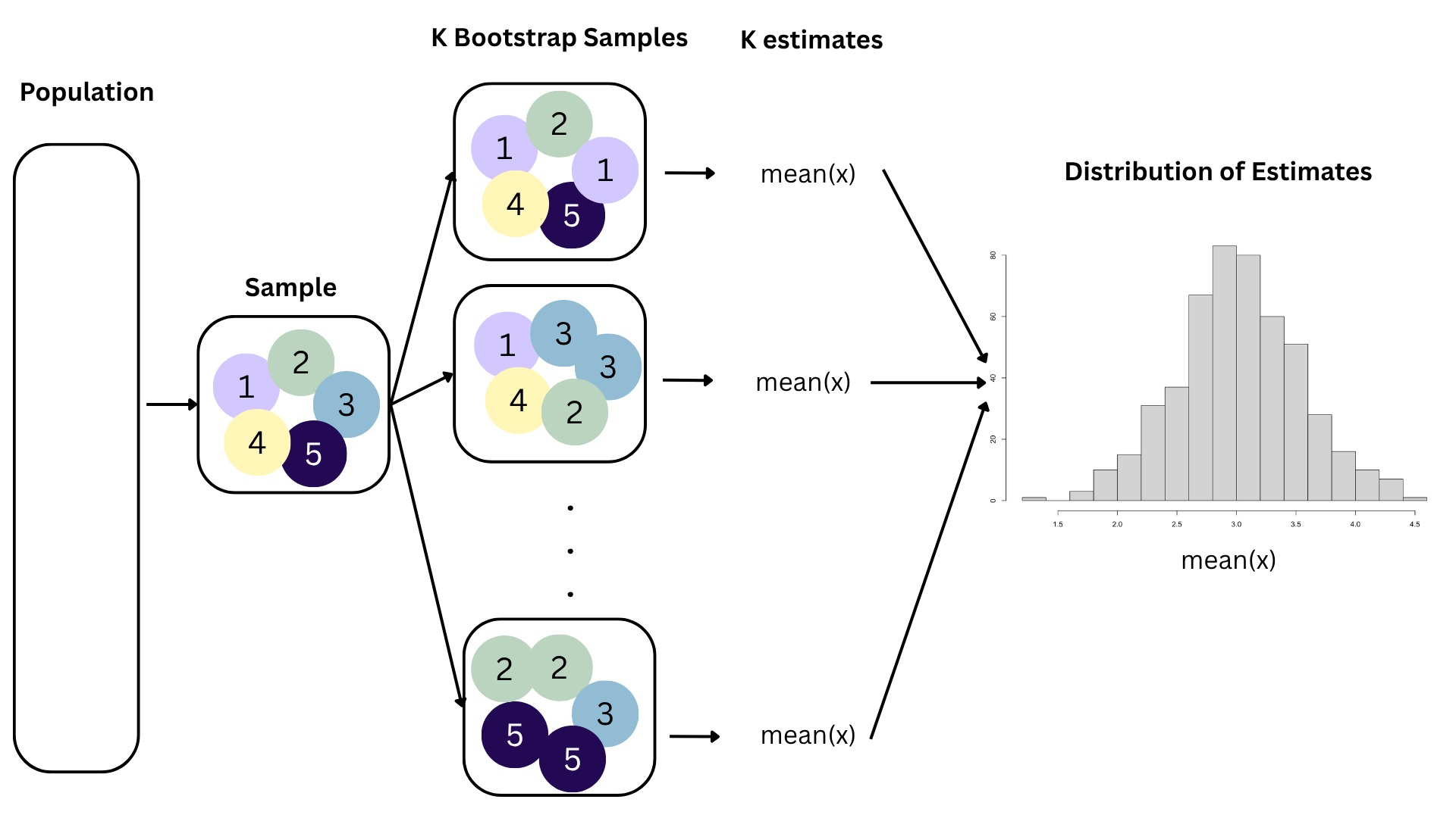
Bootstrapping
We approximate this idea of “alternative, hypothetical datasets I could have observed” by resampling our data with replacement;
-
We construct a new dataset of the same size by randomly picking rows out of the original one:
- Some rows will be duplicated;
- Some rows will not appear at all;
- Hence, the new dataset is different from the original;
- Different dataset >> different estimate;
Repeat this processes hundred or thousands of times, and observe how the estimates vary as you refit the model on alternative datasets;
This gives you a sense of the sampling variability of your estimates.
Bootstrapping
Bootstrapping
Bootstrapping
Bootstrapping
Bootstrapping
Bootstrapping
Bootstrapping
Toy: Bootstrap samples 1
Original data
# A tibble: 6 × 3
     id       x       y
  <int>   <dbl>   <dbl>
1     1  0.432   1.53
2     2 -2.01    1.80
3     3 -0.0467  1.43
4     4 -1.05    0.0518
5     5  0.327   0.820
6     6 -0.679  -0.961
Original estimates:
# A tibble: 2 × 2
  term        estimate
  <chr>          <dbl>
1 (Intercept)   0.801
2 x             0.0450
Sample with replacement:
# A tibble: 6 × 3
     id      x      y
  <int>  <dbl>  <dbl>
1     5  0.327  0.820
2     6 -0.679 -0.961
3     6 -0.679 -0.961
4     1  0.432  1.53
5     6 -0.679 -0.961
6     1  0.432  1.53
Different data >> new estimates:
# A tibble: 2 × 2
  term        estimate
  <chr>          <dbl>
1 (Intercept)    0.462
2 x              2.11
Bootstrap samples 2
Original data
# A tibble: 6 × 3
     id       x       y
  <int>   <dbl>   <dbl>
1     1  0.432   1.53
2     2 -2.01    1.80
3     3 -0.0467  1.43
4     4 -1.05    0.0518
5     5  0.327   0.820
6     6 -0.679  -0.961
Original estimates:
# A tibble: 2 × 2
  term        estimate
  <chr>          <dbl>
1 (Intercept)   0.801
2 x             0.0450
Sample with replacement:
# A tibble: 6 × 3
     id       x      y
  <int>   <dbl>  <dbl>
1     2 -2.01    1.80
2     5  0.327   0.820
3     1  0.432   1.53
4     6 -0.679  -0.961
5     3 -0.0467  1.43
6     2 -2.01    1.80
Different data >> new estimates:
# A tibble: 2 × 2
  term        estimate
  <chr>          <dbl>
1 (Intercept)    0.913
2 x             -0.236
Bootstrap samples 3
Original data
# A tibble: 6 × 3
     id       x       y
  <int>   <dbl>   <dbl>
1     1  0.432   1.53
2     2 -2.01    1.80
3     3 -0.0467  1.43
4     4 -1.05    0.0518
5     5  0.327   0.820
6     6 -0.679  -0.961
Original estimates:
# A tibble: 2 × 2
  term        estimate
  <chr>          <dbl>
1 (Intercept)   0.801
2 x             0.0450
Sample with replacement:
# A tibble: 6 × 3
     id      x      y
  <int>  <dbl>  <dbl>
1     6 -0.679 -0.961
2     1  0.432  1.53
3     5  0.327  0.820
4     6 -0.679 -0.961
5     6 -0.679 -0.961
6     5  0.327  0.820
Different data >> new estimates:
# A tibble: 2 × 2
  term        estimate
  <chr>          <dbl>
1 (Intercept)    0.357
2 x              1.96
Interval estimation
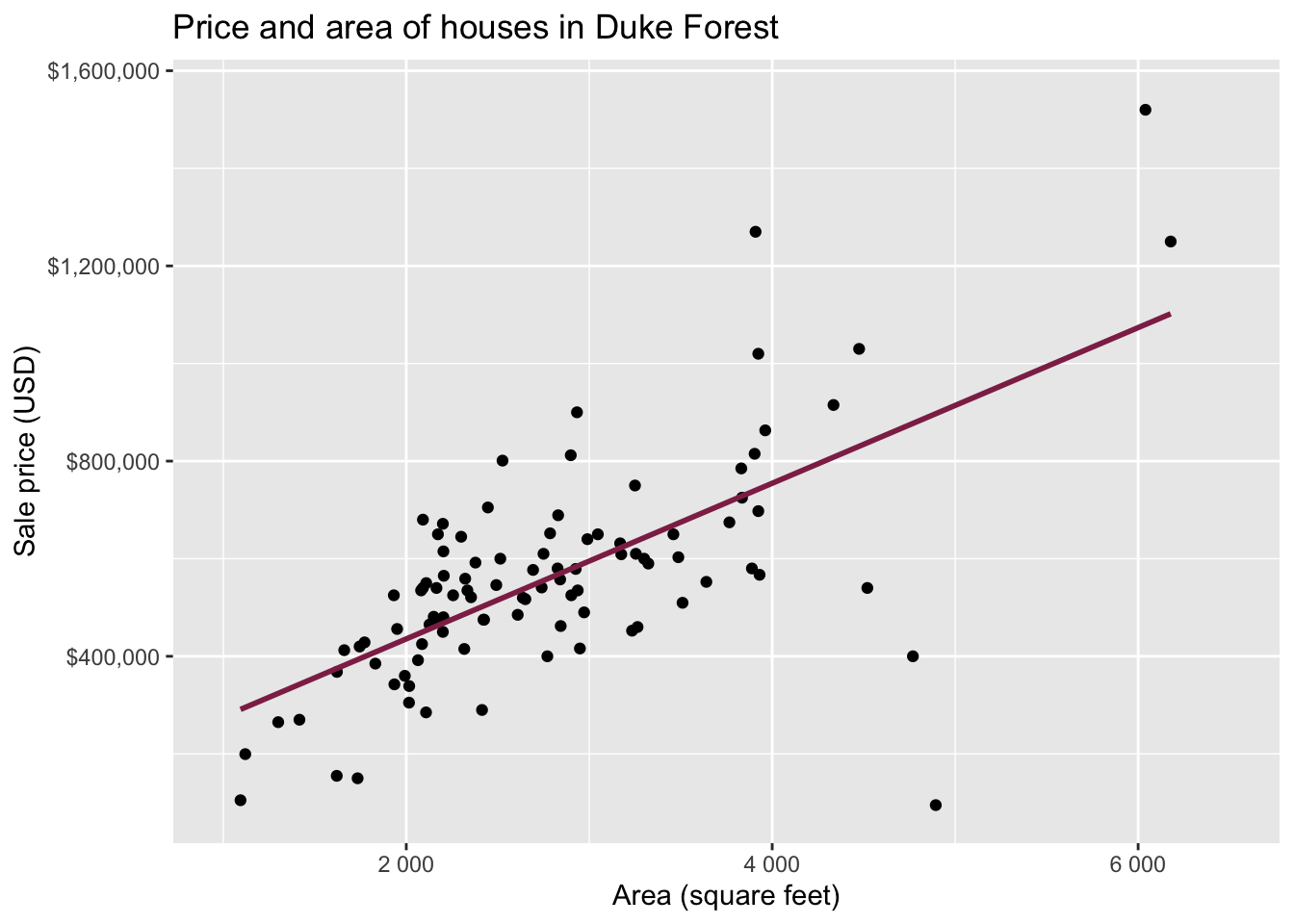
Data: Houses in Duke Forest
- Data on houses that were sold in the Duke Forest neighborhood of Durham, NC around November 2020
- Scraped from Zillow
- Source:
openintro::duke_forest

Goal: Use the area (in square feet) to understand variability in the price of houses in Duke Forest.
Exploratory data analysis
Code
ggplot(duke_forest, aes(x = area, y = price)) +
  geom_point(alpha = 0.7) +
  labs(
    x = "Area (square feet)",
    y = "Sale price (USD)",
    title = "Price and area of houses in Duke Forest"
  ) +
scale_y_continuous(labels = label_dollar()) 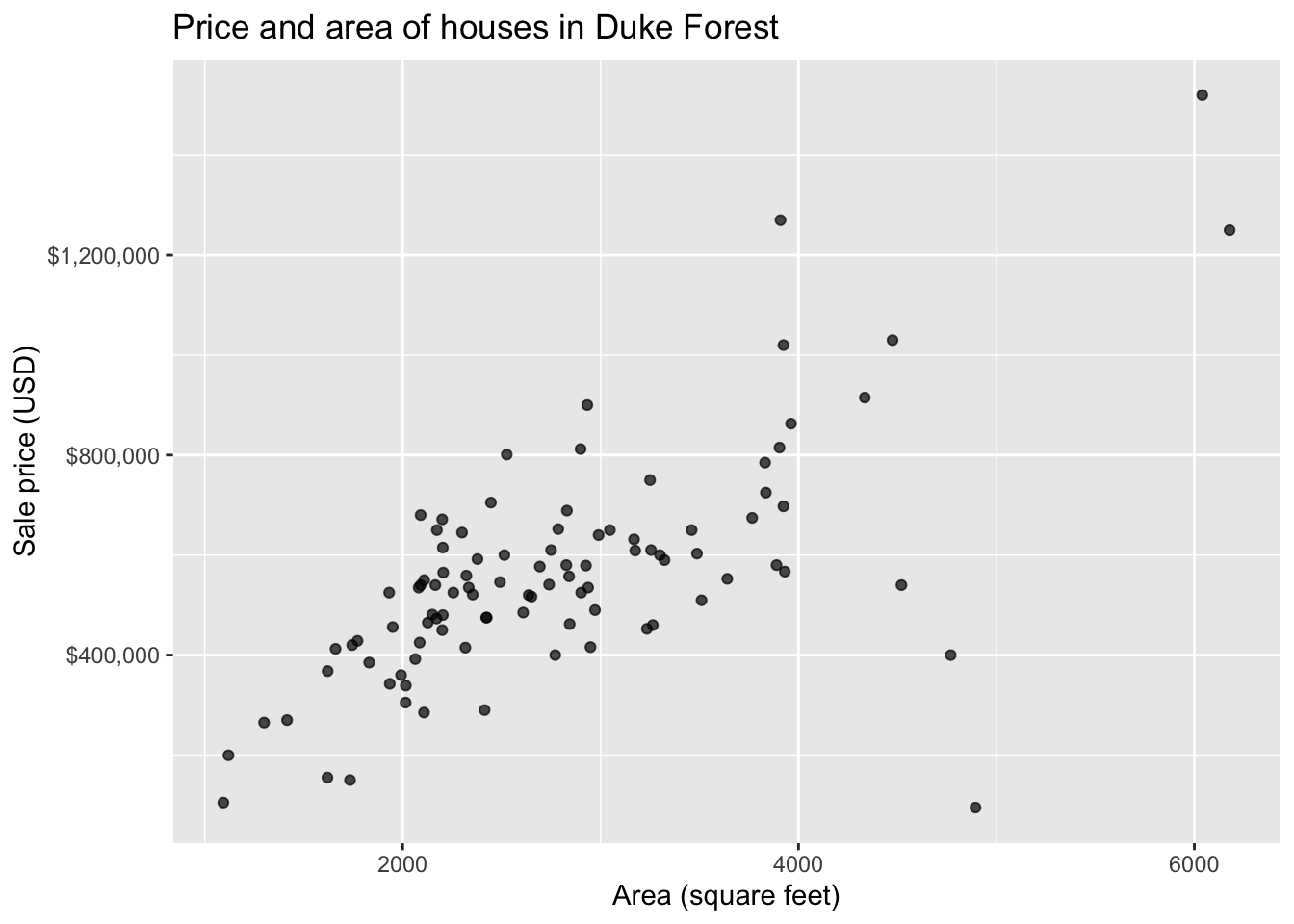
Modeling
df_fit <- linear_reg() |>
  fit(price ~ area, data = duke_forest)

tidy(df_fit) |>
kable(digits = 2) # neatly format table to 2 digits| term | estimate | std.error | statistic | p.value |
|---|---|---|---|---|
| (Intercept) | 116652.33 | 53302.46 | 2.19 | 0.03 |
| area | 159.48 | 18.17 | 8.78 | 0.00 |
. . .
-
Intercept: Duke Forest houses that are 0 square feet are expected to sell, for $116,652, on average.
- Is this interpretation useful?
- Slope: For each additional square foot, we expect the sale price of Duke Forest houses to be higher by $159, on average.
From sample to population
For each additional square foot, we expect the sale price of Duke Forest houses to be higher by $159, on average.
- This estimate is valid for the single sample of 98 houses.
- But what if we’re not interested quantifying the relationship between the size and price of a house in this single sample?
- What if we want to say something about the relationship between these variables for all houses in Duke Forest?
Statistical inference
Statistical inference provide methods and tools so we can use the single observed sample to make valid statements (inferences) about the population it comes from
For our inferences to be valid, the sample should be random and representative of the population we’re interested in

Inference for simple linear regression
Calculate a confidence interval for the slope, \(\beta_1\) (today)
Conduct a hypothesis test for the slope, \(\beta_1\) (Thursday)
Confidence interval
- A plausible range of values for a population parameter is called a confidence interval
- Using only a single point estimate is like fishing in a murky lake with a spear, and using a confidence interval is like fishing with a net
- We can throw a spear where we saw a fish but we will probably miss, if we toss a net in that area, we have a good chance of catching the fish
- Similarly, if we report a point estimate, we probably will not hit the exact population parameter, but if we report a range of plausible values we have a good shot at capturing the parameter
Confidence interval for the slope
A confidence interval will allow us to make a statement like “For each additional square foot, the model predicts the sale price of Duke Forest houses to be higher, on average, by $159, plus or minus X dollars.”
. . .
Should X be $10? $100? $1000?
If we were to take another sample of 98 would we expect the slope calculated based on that sample to be exactly $159? Off by $10? $100? $1000?
The answer depends on how variable (from one sample to another sample) the sample statistic (the slope) is
We need a way to quantify the variability of the sample statistic
Quantify the variability of the slope
for estimation
- Two approaches:
- Via simulation (what we’ll do in this course)
- Via mathematical models (what you can learn about in future courses)
-
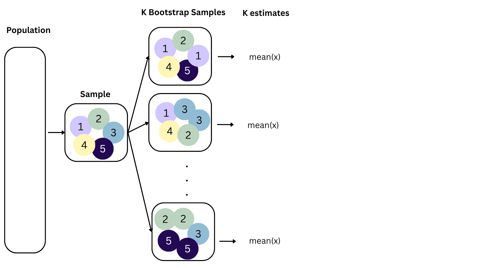
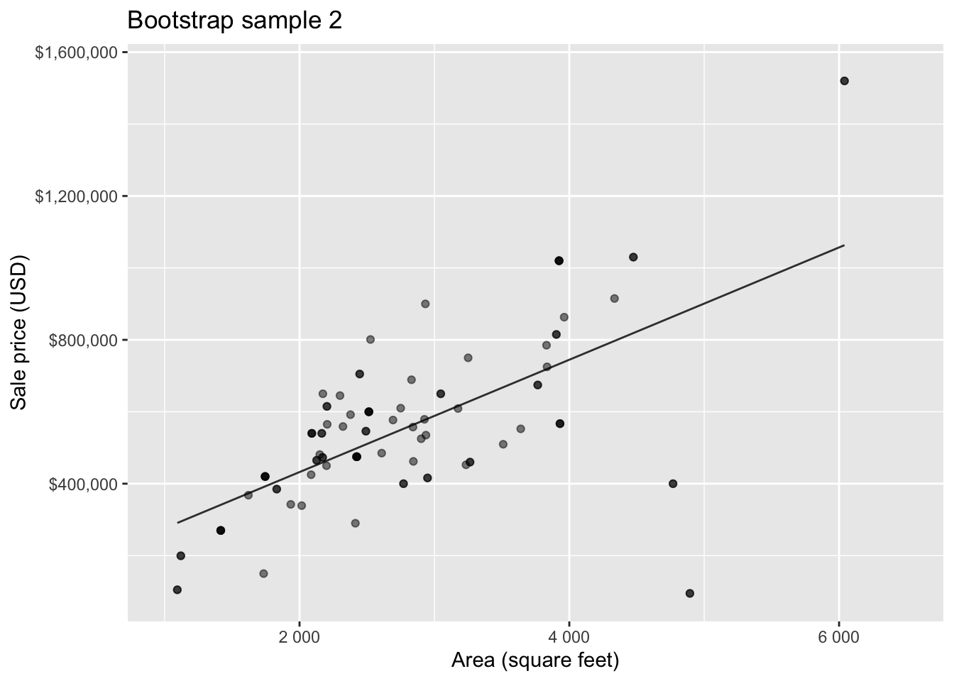
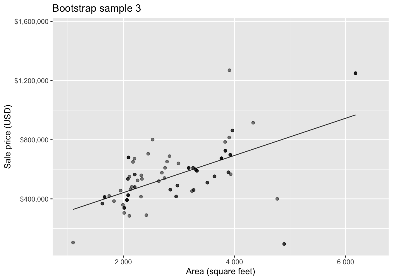
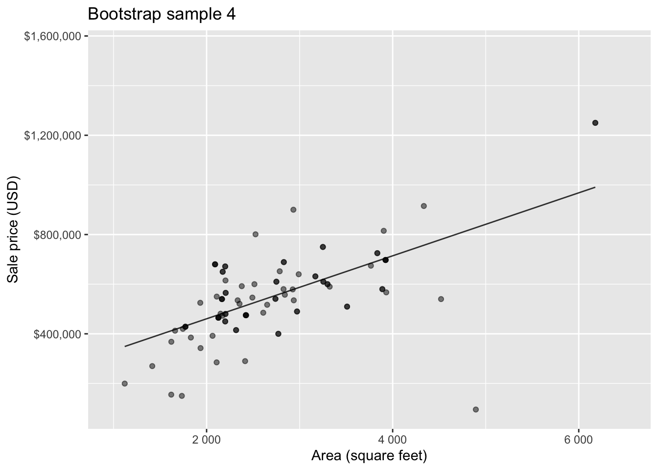
Bootstrapping to quantify the variability of the slope for the purpose of estimation:
- Bootstrap new samples from the original sample
- Fit models to each of the samples and estimate the slope
- Use features of the distribution of the bootstrapped slopes to construct a confidence interval
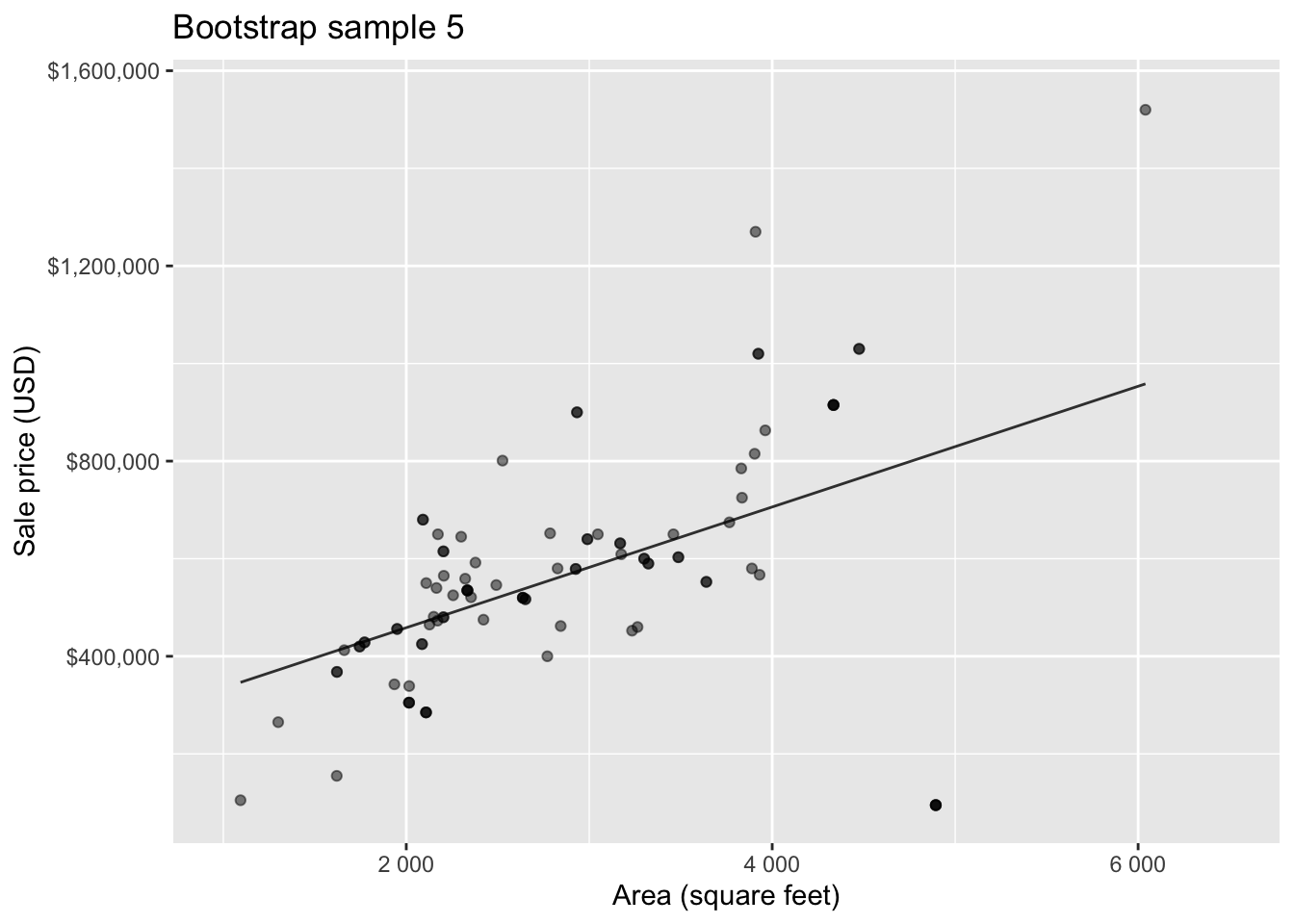
Bootstrap sample 1


Bootstrap sample 2

Bootstrap sample 3

Bootstrap sample 4

Bootstrap sample 5
. . .
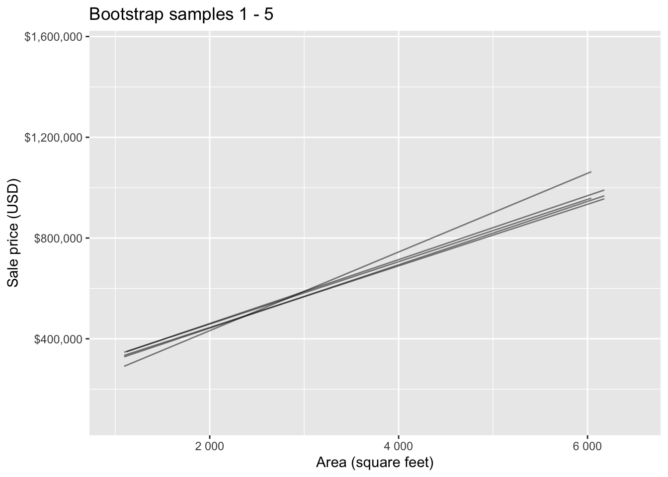
so on and so forth…
Bootstrap samples 1 - 5

Bootstrap samples 1 - 100

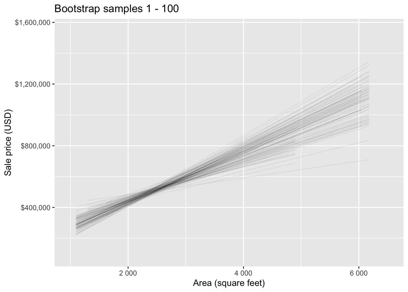
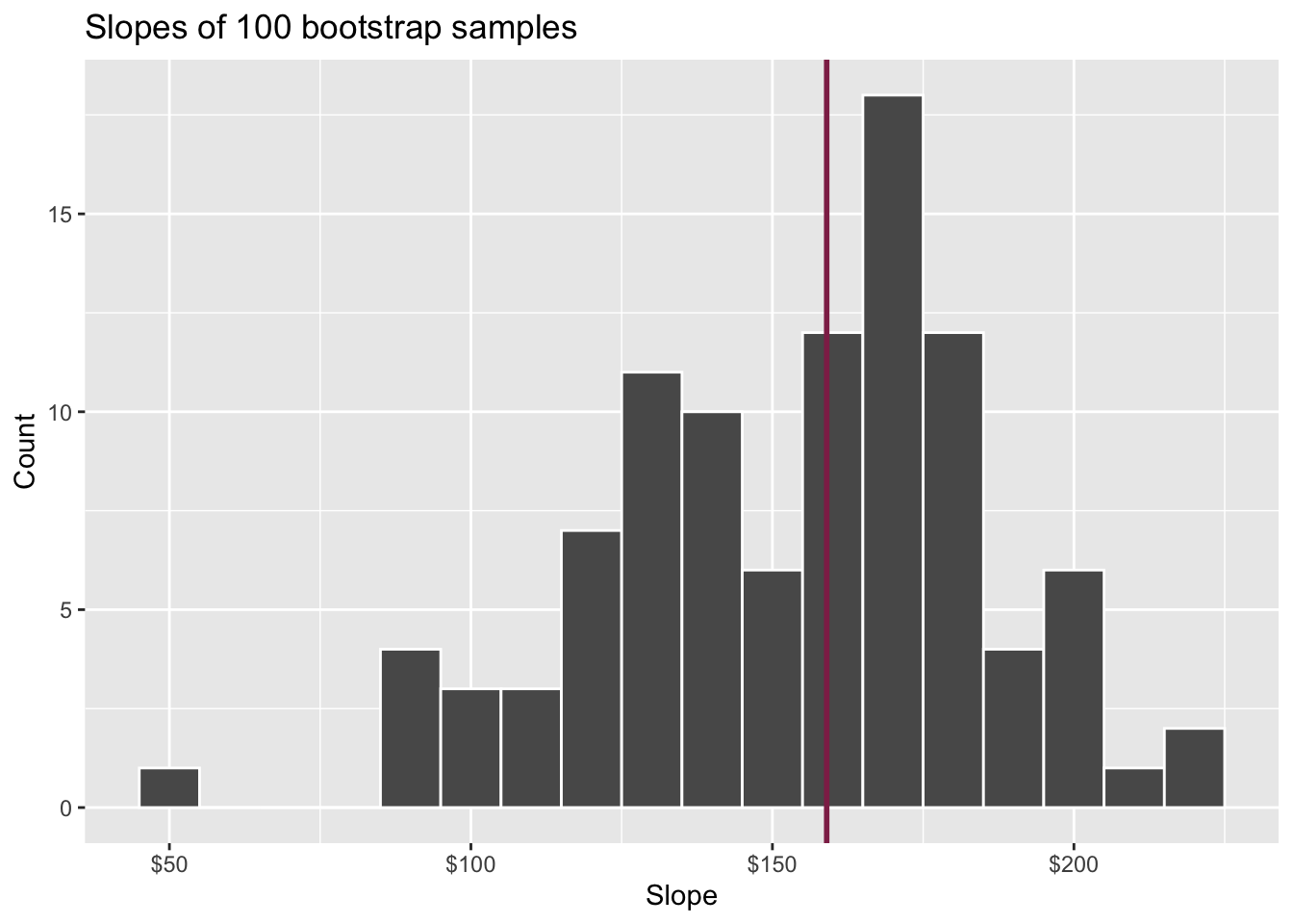
Slopes of bootstrap samples
Fill in the blank: For each additional square foot, the model predicts the sale price of Duke Forest houses to be higher, on average, by $159, plus or minus ___ dollars.
Slopes of bootstrap samples
Fill in the blank: For each additional square foot, we expect the sale price of Duke Forest houses to be higher, on average, by $159, plus or minus ___ dollars.

Confidence level
How confident are you that the true slope is between $0 and $250? How about $150 and $170? How about $90 and $210?
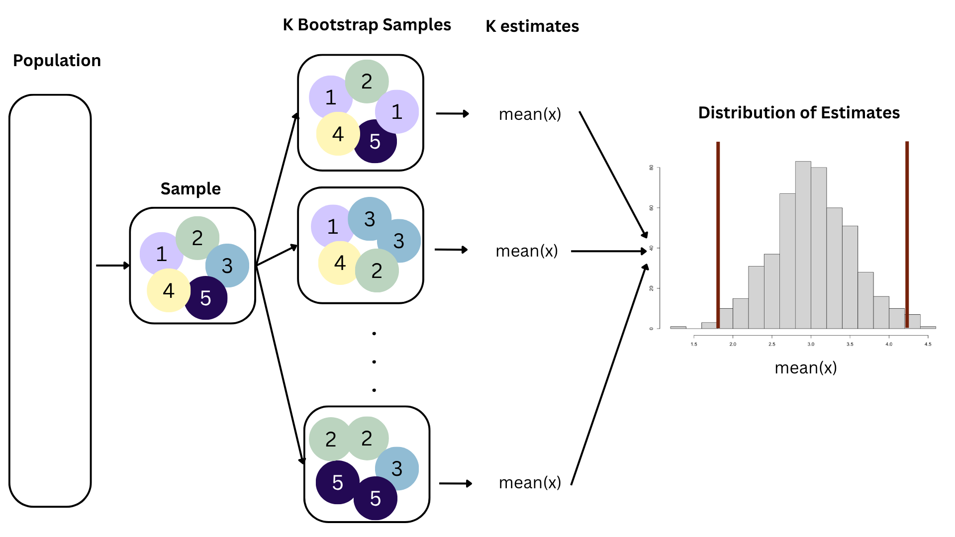
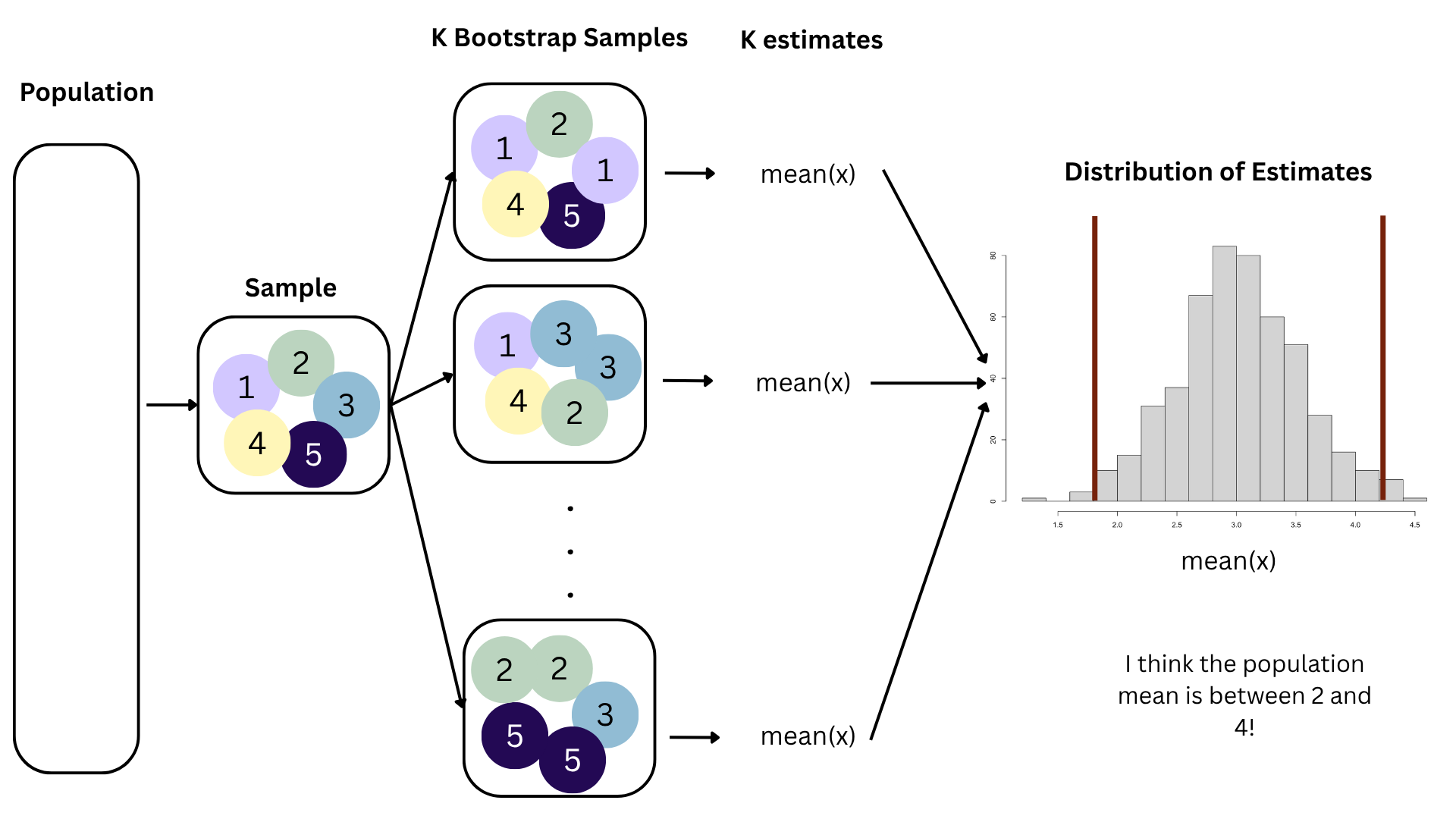
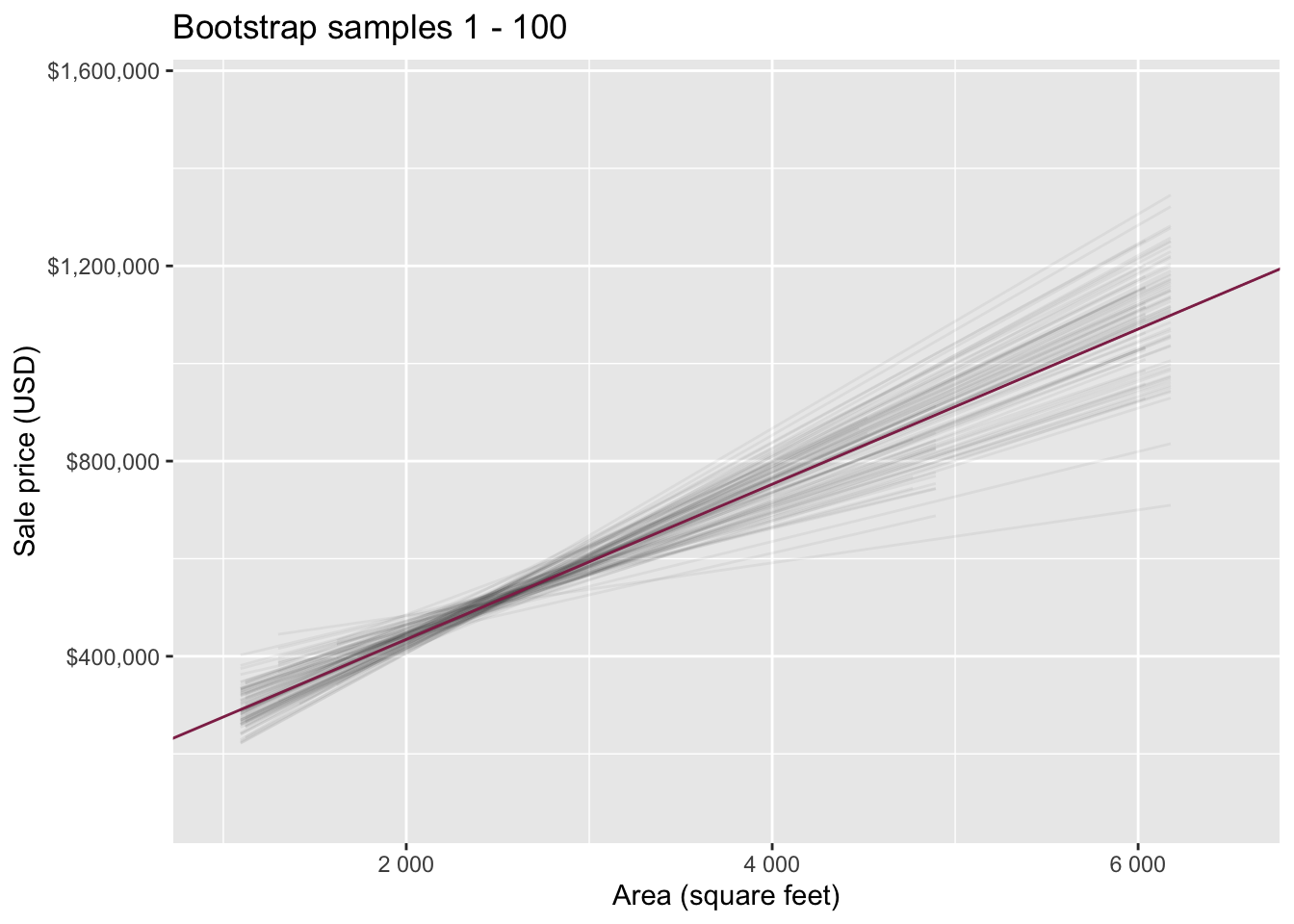
95% confidence interval
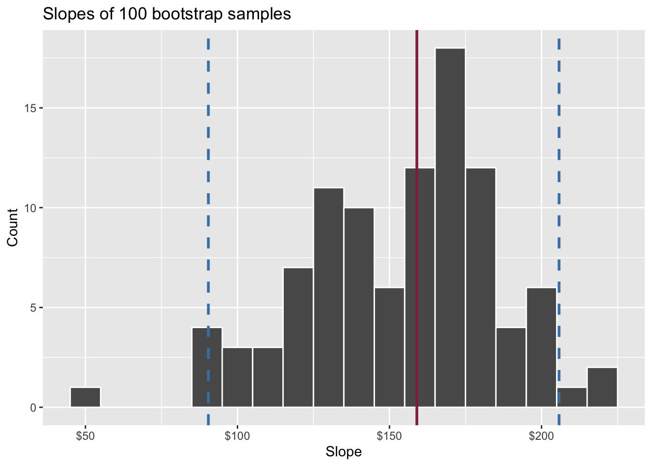
- A 95% confidence interval is bounded by the middle 95% of the bootstrap distribution
- We are 95% confident that for each additional square foot, the model predicts the sale price of Duke Forest houses to be higher, on average, by $90.43 to $205.77.
Where do the bounds come from?
Quantiles!
Think IQR! 50% of the bootstrap distribution is between the 25% quantile on the left and the 75% quantile on the right. But we want more than 50%
90% of the bootstrap distribution is between the 5% quantile on the left and the 95% quantile on the right;
95% of the bootstrap distribution is between the 2.5% quantile on the left and the 97.5% quantile on the right;
And so on.
Application exercise
ae-22-duke-forest-bootstrap
Go to your ae project in RStudio.
If you haven’t yet done so, make sure all of your changes up to this point are committed and pushed, i.e., there’s nothing left in your Git pane.
If you haven’t yet done so, click Pull to get today’s application exercise file: ae-22-duke-forest-bootstrap.qmd.
Work through the application exercise in class, and render, commit, and push your edits.
Computing the CI for the slope I
Calculate the observed slope:
observed_fit <- duke_forest |>
  specify(price ~ area) |>
  fit()

observed_fit
# A tibble: 2 × 2
term estimate
<chr> <dbl>
1 intercept 116652.
2 area 159.Computing the CI for the slope II
Take 100 bootstrap samples and fit models to each one:
set.seed(1120)

boot_fits <- duke_forest |>
  specify(price ~ area) |>
  generate(reps = 100, type = "bootstrap") |>
  fit()

boot_fits
# A tibble: 200 × 3
# Groups: replicate [100]
replicate term estimate
<int> <chr> <dbl>
1 1 intercept 47819.
2 1 area 191.
3 2 intercept 144645.
4 2 area 134.
5 3 intercept 114008.
6 3 area 161.
7 4 intercept 100639.
8 4 area 166.
9 5 intercept 215264.
10 5 area 125.
# ℹ 190 more rowsComputing the CI for the slope III
Percentile method: Compute the 95% CI as the middle 95% of the bootstrap distribution:
Precision vs. accuracy
If we want to be very certain that we capture the population parameter, should we use a wider or a narrower interval? What drawbacks are associated with using a wider interval?
. . .

Precision vs. accuracy
How can we get best of both worlds – high precision and high accuracy?
Changing confidence level
How would you modify the following code to calculate a 90% confidence interval? How would you modify it for a 99% confidence interval?
Changing confidence level
## confidence level: 90%
get_confidence_interval(
  boot_fits, point_estimate = observed_fit,
  level = 0.90, type = "percentile"
)
# A tibble: 2 × 3
term lower_ci upper_ci
<chr> <dbl> <dbl>
1 area 104. 212.
2 intercept -24380. 256730.## confidence level: 99%
get_confidence_interval(
boot_fits, point_estimate = observed_fit,
level = 0.99, type = "percentile"
)# A tibble: 2 × 3
term lower_ci upper_ci
<chr> <dbl> <dbl>
1 area 56.3 226.
2 intercept -61950. 370395.Recap
Population: Complete set of observations of whatever we are studying, e.g., people, tweets, photographs, etc. (population size = \(N\))
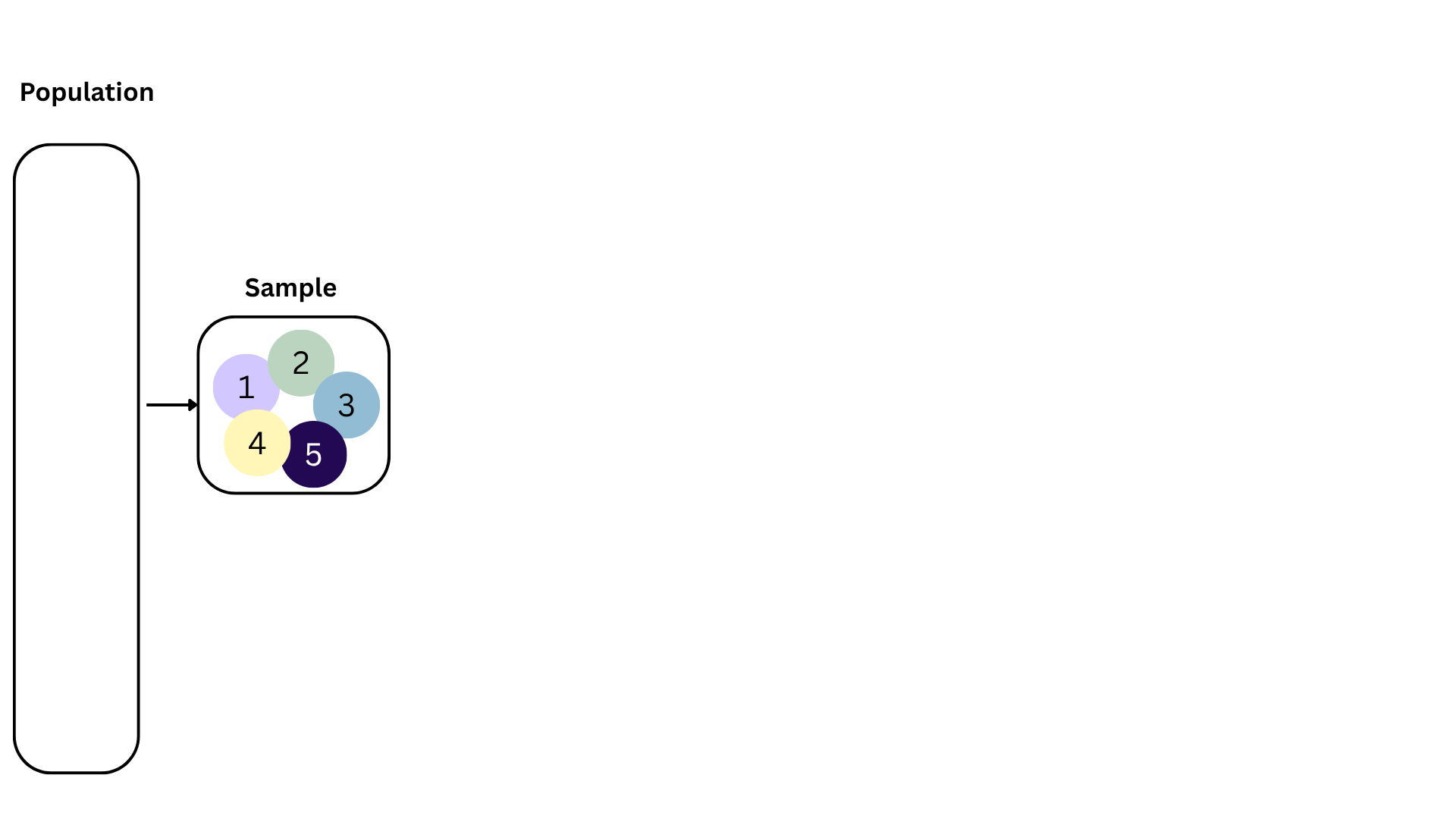
Sample: Subset of the population, ideally random and representative (sample size = \(n\))
Sample statistic \(\ne\) population parameter, but if the sample is good, it can be a good estimate
Statistical inference: Discipline that concerns itself with the development of procedures, methods, and theorems that allow us to extract meaning and information from data that has been generated by stochastic (random) process
We report the estimate with a confidence interval, and the width of this interval depends on the variability of sample statistics from different samples from the population
Since we can’t continue sampling from the population, we bootstrap from the one sample we have to estimate sampling variability